Although probiotics' main known effects are in the digestive system, over the last years several benefits that come from their topical use, have been investigated. Several studies have reported beneficial effects on different skin disorders, such as atopic dermatitis, acne, eczema, psoriasis, wound healing, skin aging and reactive skin. Their main action is assigned to the inhibition of skin colonization by pathogens. In this work, the growths of three probiotic strains were evaluated in the presence of abiotic factors similar to those found in skin, namely, UV radiation, temperature, pH, NaCl and fatty acids. Lactobacillus rhamnosus showed increased growth under the pH of 6, but no differences in its growth were found for the various NaCl concentrations tested. Lactobacillus delbrueckii increased the number of bacterial cells in 88.8% when grown in 10 mM NaCl concentration, while Propioniferax innocua showed increased growth at 45 °C. All tested probiotic bacteria were able to grow under skin-like conditions. However, L. rhamnosus was the probiotic that showed the best results. The results obtained in this study indicate that the used probiotics may be beneficial in the treatment of skin diseases, since they are able to successfully thrive in skin-like conditions.
Citation: MP Lizardo, FK Tavaria. Probiotic growth in skin-like conditions[J]. AIMS Microbiology, 2022, 8(4): 388-402. doi: 10.3934/microbiol.2022027
Although probiotics' main known effects are in the digestive system, over the last years several benefits that come from their topical use, have been investigated. Several studies have reported beneficial effects on different skin disorders, such as atopic dermatitis, acne, eczema, psoriasis, wound healing, skin aging and reactive skin. Their main action is assigned to the inhibition of skin colonization by pathogens. In this work, the growths of three probiotic strains were evaluated in the presence of abiotic factors similar to those found in skin, namely, UV radiation, temperature, pH, NaCl and fatty acids. Lactobacillus rhamnosus showed increased growth under the pH of 6, but no differences in its growth were found for the various NaCl concentrations tested. Lactobacillus delbrueckii increased the number of bacterial cells in 88.8% when grown in 10 mM NaCl concentration, while Propioniferax innocua showed increased growth at 45 °C. All tested probiotic bacteria were able to grow under skin-like conditions. However, L. rhamnosus was the probiotic that showed the best results. The results obtained in this study indicate that the used probiotics may be beneficial in the treatment of skin diseases, since they are able to successfully thrive in skin-like conditions.

| [1] |
Chiller K, Selkin BA, Murakawa GJ (2001) Skin microflora and bacterial infections of the skin. J Invest Dermatol Symp Proc 6: 170-174. https://doi.org/10.1046/j.0022-202x.2001.00043.x 
|
| [2] |
Kendall AC, Kiezel-Tsugunova M, Brownbridge LC, et al. (2017) Lipid functions in skin: Differential effects of n-3 polyunsaturated fatty acids on cutaneous ceramides, in a human skin organ culture model. Biochim Biophys Acta Biomembr 1859: 1679-1689. https://doi.org/10.1016/j.bbamem.2017.03.016
|
| [3] |
Losquadro WD (2017) Anatomy of the skin and the pathogenesis of nonmelanoma skin cancer. Facial Plast Surg Clin North Am 25: 283-289. https://doi.org/10.1016/j.fsc.2017.03.001
|
| [4] | Prince T (2012) Evaluation of the utility of probiotics for the prevention of infections in a model of the skin. PhD thesis, University of Manchester . |
| [5] |
Grice EA, Kong HH, Renaud G, et al. (2008) A diversity profile of the human skin microbiota. Genome Res 18: 1043-1050. https://doi.org/10.1101/gr.075549.107
|
| [6] |
Kong HH, Segre JA (2012) Skin microbiome: looking back to move forward. J Inv Dermatol 132: 933-939. https://doi.org/10.1038/jid.2011.417
|
| [7] |
Grice EA, Kong HH, Conlan S, et al. (2009) Topographical and temporal diversity of the human skin microbiome. Science 324: 1190-1192. https://doi.org/10.1126/science.1171700
|
| [8] |
Grice EA, Segre JA (2011) The skin microbiome. Nat Rev Microbiol 9: 244-253. https://doi.org/10.1038/nrmicro2537
|
| [9] |
Al-Ghazzewi FH, Tester RF (2014) Impact of prebiotics and probiotics on skin health. Benef Microbes 5: 99-107. https://doi.org/10.3920/BM2013.0040
|
| [10] |
Zommiti M, Feuilloley MGJ, Connil N (2020) Update of probiotics in human world: A nonstop source of benefactions till the end of time. Microorganisms 30: 1907. https://doi.org/10.3390/microorganisms8121907
|
| [11] |
Lee CH, Wu SB, Hong CH, et al. (2013) Molecular mechanisms of UV-induced apoptosis and its effects on skin residential cells: the implication in UV-based phototherapy. Int J Mol Sci 14: 6414-6435. https://doi.org/10.3390/ijms14036414
|
| [12] |
Coohill TP, Sagripanti JL (2009) Bacterial inactivation by solar ultraviolet radiation compared with sensitivity to 254 nm radiation. Photochem Photobiol 85: 1043-1052. https://doi.org/10.1111/j.1751-1097.2009.00586.x
|
| [13] | Patra VK, Byrne SN, Wolf P (2016) The skin microbiome: is it affected by UV-induced immune suppression?. Front Microbiol 7: 1-11. https://doi.org/10.3389/fmicb.2016.01235 |
| [14] |
Souak D, Barreau M, Courtois A, et al. (2021) Challenging cosmetic innovation: the skin microbiota and probiotics protect the skin from UV-induced damage. Microorganisms 27: 936. https://doi.org/10.3390/microorganisms9050936
|
| [15] |
Cinque B, La Torre C, Melchiorre E, et al. (2011) Use of probiotics for dermal applications in probiotics. Probiotics . Berlin: Springer 221-241. https://doi.org/10.1007/978-3-642-20838-6_9
|
| [16] |
Ali SM, Yosipovitch G (2013) Skin pH: From basic science to basic skin care. Acta Dermato-Venereologica 93: 261-267. https://doi.org/10.2340/00015555-1531
|
| [17] |
Lambers H, Piessens S, Bloem A, et al. (2006) Natural skin surface pH is on average below 5, which is beneficial for its resident flora. Int J Cosmet Sci 28: 359-370. https://doi.org/10.1111/j.1467-2494.2006.00344.x
|
| [18] |
Gläser R, Harder J, Lange H, et al. (2005) Antimicrobial psoriasin (S100A7) protects human skin from Escherichia coli infection. Nat Immunol 6: 57-64. https://doi.org/10.1038/ni1142
|
| [19] |
Matthias J, Maul J, Noster R, et al. (2019) Sodium chloride is an ionic checkpoint for human TH2 cells and shapes the atopic skin microenvironment. Sci Transl Med 11: 1-11. https://doi.org/10.1126/scitranslmed.aau0683
|
| [20] |
Lloyd CM, Snelgrove RJ (2018) Type 2 immunity: Expanding our view. Sci Immunol 3: eaat1604. https://doi.org/10.1126/sciimmunol.aat1604
|
| [21] |
Liu Y, Wang L, Liu J, et al. (2013) A study of human skin and surface temperatures in stable and unstable thermal environments. J Therm Biol 38: 440-448. https://doi.org/10.1016/j.jtherbio.2013.06.006
|
| [22] |
Huus KE, Ley RE (2021) Blowing hot and cold: body temperature and the microbiome. mSystems 6: e0070721. https://doi.org/10.1128/mSystems.00707-21
|
| [23] |
Mieremet A, Helder R, Nadaban A, et al. (2019) Contribution of palmitic acid to epidermal morphogenesis and lipid barrier formation in human skin equivalent. Int J Mol Sci 20: 1-18. https://doi.org/10.3390/ijms20236069
|
| [24] |
Picardo M, Ottaviani M, Camera E, et al. (2009) Sebaceous gland lipids. Dermato-Endocrinol 1: 68-71. https://doi.org/10.4161/derm.1.2.8472
|
| [25] |
Kim EJ, Kim MK, Jin XJ, et al. (2010) Skin aging and photoaging alter fatty acids composition, including 11,14,17-eicosatrienoic acid, in the epidermis of human skin. J Korean Med Sci 25: 980-983. https://doi.org/10.3346/jkms.2010.25.6.980
|
| [26] |
Vičanová J, Weerheim AM, Kempenaar JA, et al. (1999) Incorporation of linoleic acid by cultured human keratinocytes. Arch Dermatol Res 291: 405-412. https://doi.org/10.1007/s004030050430
|
| [27] |
Gascón J, Oubiña A, Pérez-Lezaun A, et al. (1995) Sensitivity of selected bacterial species to UV radiation. Curr Microbiol 30: 177-182. https://doi.org/10.1007/BF00296205
|
| [28] |
Diffey BL (2002) Sources and measurement of ultraviolet radiation. Methods 28: 4-13. https://doi.org/10.1016/S1046-2023(02)00204-9
|
| [29] |
Jin Q, Kirk MF (2018) pH as a primary control in environmental microbiology: 1. thermodynamic perspective. Front Environ Sci 6: 1-15. https://doi.org/10.3389/fenvs.2018.00021
|
| [30] | Jenkinson D (1993) The basis of the skin surface ecosystem. The skin microflora and microbial skin disease . Cambridge: Cambridge University Press 1-32. https://doi.org/10.1017/CBO9780511527012.002 |
| [31] |
Dréno B, Araviiskaia E, Berardesca E, et al. (2016) Microbiome in healthy skin, update for dermatologists. J Eur Acad Dermatol Venereol 30: 2038-2047. https://doi.org/10.1111/jdv.13965
|
| [32] |
Zotta T, Ricciardi A, Ianniello R, et al. (2014) Assessment of aerobic and respiratory growth in the Lactobacillus casei group. PLoS One 9: e99189. https://doi.org/10.1371/journal.pone.0099189
|
| [33] |
Marty-Teysset C, De La Torre F, Garel JR (2000) Increased production of hydrogen peroxide by Lactobacillus delbrueckii subsp. bulgaricus upon aeration: involvement of an NADH oxidase in oxidative stress. Appl Environ Microbiol 66: 262-267. https://doi.org/10.1128/AEM.66.1.262-267.2000
|
| [34] |
Shin D, Lee Y, Huang, YH, et al. (2018) Probiotic fermentation augments the skin anti-photoaging properties of Agastache rugosa through up-regulating antioxidant components in UV-B-irradiated HaCaT keratinocytes. BMC Complement Altern Med 18: 1-10. https://doi.org/10.1186/s12906-018-2194-9
|
| [35] | Valík L, Medvedová A, Liptáková D (2008) Characterization of the growth of Lactobacillus rhamnosus GG in milk at suboptimal temperatures. J Food Nutr Res 47: 60-67. |
| [36] |
Beal C, Louvet P, Corrieu G (1989) Influence of controlled pH and temperature on the growth and acidification of pure cultures of Streptococcus thermophilus 404 and Lactobacillus bulgaricus 398. Appl Microbiol Biotechnol 32: 148-154. https://doi.org/10.1007/BF00165879
|
| [37] |
Stevenson K, McVey A, Clark I, et al. (2016) General calibration of microbial growth in microplate readers. Sci Rep 6: 38828. https://doi.org/10.1038/srep38828
|
| [38] |
Prasad J, McJarrow P, Gopal P (2003) Heat and osmotic stress responses of probiotic Lactobacillus rhamnosus HN001 (DR20) in relation to viability after drying. Appl Environ Microbiol 69: 917-925. https://doi.org/10.1128/AEM.69.2.917-925.2003
|
| [39] | Chun L, Li-Bo L, Di S, et al. (2012) Response of osmotic adjustment of Lactobacillus bulgaricus to NaCl stress. J Northeast Agri Univ 19: 66-74. https://doi.org/10.1016/S1006-8104(13)60054-9 |
| [40] |
Yokota A, Tamura T, Takeuchi M, et al. (1994) Transfer of Propionibacterium innocuum pitcher and collins 1991 to propioniferax gen. nov. as Propioniferax innocua comb. nov. Int J Syst Bacteriol 44: 579-582. https://doi.org/10.1099/00207713-44-3-579
|
| [41] | Yokota A (2015) The genus propioniferax. Bergey's Manual of Systematic Bacteriology 1-4. https://doi.org/10.1002/9781118960608.gbm00170 |
| [42] |
Partanen L, Marttinen N, Alatossava T (2001) Fats and fatty acids as growth factors for Lactobacillus delbrueckii. Sys Appl Microbiol 24: 500-506. https://doi.org/10.1078/0723-2020-00078
|


Figures(6)

MP Lizardo, FK Tavaria. Probiotic growth in skin-like conditions[J]. AIMS Microbiology, 2022, 8(4): 388-402. doi: 10.3934/microbiol.2022027

 ), Lactobacillus delbrueckii subsp. bulgaricus (
 ) and Propioniferax innocua (
 )
)
 ), Lactobacillus delbrueckii subsp. bulgaricus (
 ) and Propioniferax innocua (
 )
)
 ), pH 4 (
 ), pH 5 (
 ), pH 6 (
 ), pH 7 (
 ) and control (
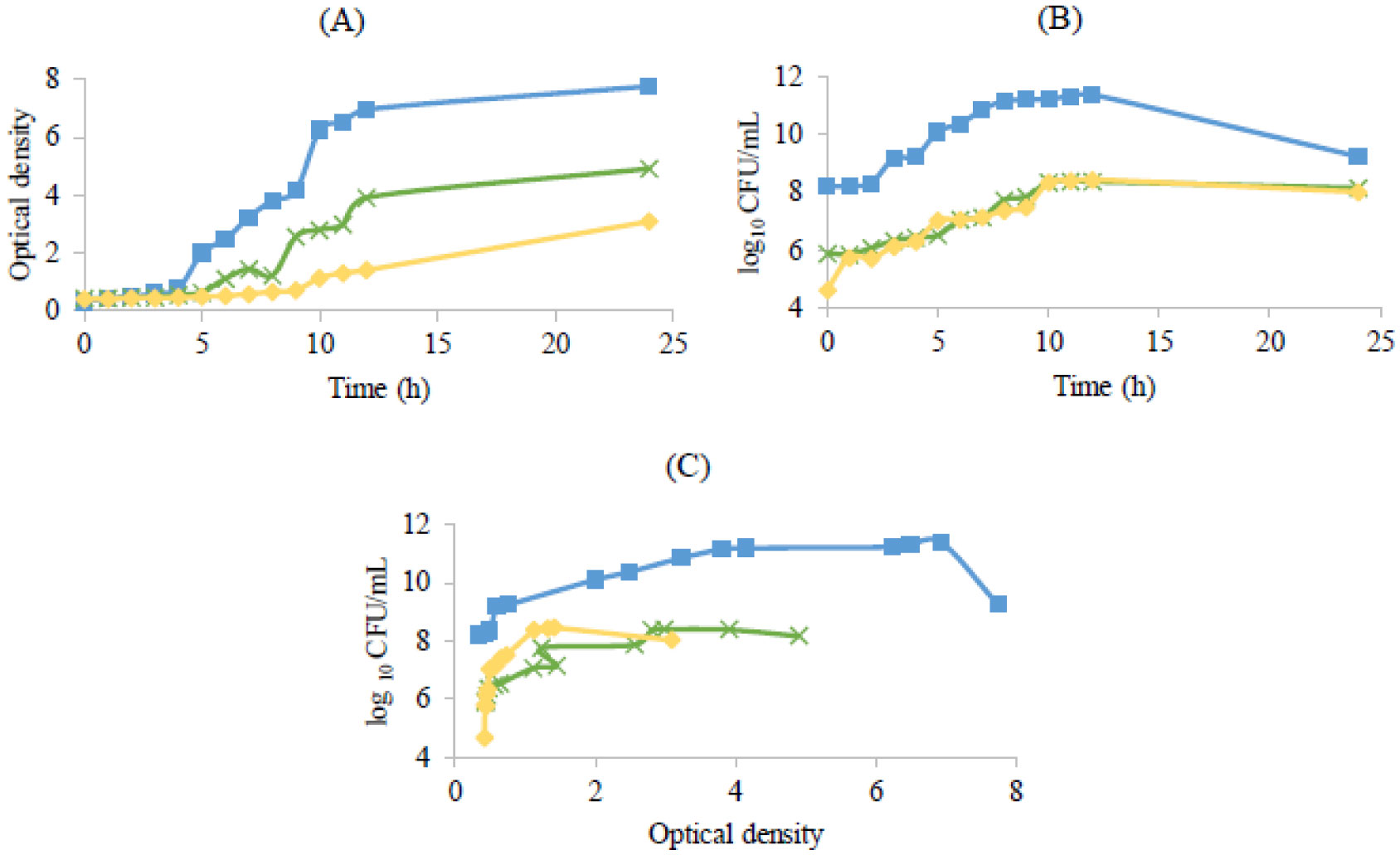
 ) during 24 hours. (A) Lactobacillus rhamnosus, (B) Lactobacillus delbrueckii subsp. bulgaricus and (C) Propioniferax innocua. Error bars are ± standard deviation
), 20 mM (), 40 mM (), 60 mM (), 80 mM () and control () during 24 hours. (A) Lactobacillus rhamnosus, (B) Lactobacillus delbrueckii subsp. bulgaricus and (C) Propioniferax innocua. Error bars are ± standard deviation
), 25 °C (), 45 °C () and control at 37 °C () during 24 hours. (A) Lactobacillus rhamnosus, (B) Lactobacillus delbrueckii subsp. bulgaricus and (C) Propioniferax innocua. Error bars are ± standard deviation
), palmitic acid 9% (), linoleic acid plus palmitic acid 15% () and control () during 24 hours. (A) Lactobacillus rhamnosus, (B) Lactobacillus delbrueckii subsp. bulgaricus and (C) Propioniferax innocua. Error bars are ± standard deviation
) during 24 hours. (A) Lactobacillus rhamnosus, (B) Lactobacillus delbrueckii subsp. bulgaricus and (C) Propioniferax innocua. Error bars are ± standard deviation
), 20 mM (), 40 mM (), 60 mM (), 80 mM () and control () during 24 hours. (A) Lactobacillus rhamnosus, (B) Lactobacillus delbrueckii subsp. bulgaricus and (C) Propioniferax innocua. Error bars are ± standard deviation
), 25 °C (), 45 °C () and control at 37 °C () during 24 hours. (A) Lactobacillus rhamnosus, (B) Lactobacillus delbrueckii subsp. bulgaricus and (C) Propioniferax innocua. Error bars are ± standard deviation
), palmitic acid 9% (), linoleic acid plus palmitic acid 15% () and control () during 24 hours. (A) Lactobacillus rhamnosus, (B) Lactobacillus delbrueckii subsp. bulgaricus and (C) Propioniferax innocua. Error bars are ± standard deviation


 DownLoad: