
In this paper, we study a model of opinion dynamics based on the so-called "bounded confidence" principle introduced by Hegselmann and Krause. Following this principle, voters participating in an electoral decision with two options are influenced by individuals sharing an opinion similar to their own.
We consider a modification of this model where the operator generating the dynamical system which describes the process of formation the final distribution of opinions in the society is defined in two steps. First, to the opinion of an agent, a value proportional to opinions in his/her "influence group" is added, and then the elements of the resulting array are divided by the maximal absolute value of elements to keep the opinions in the prescribed interval. We show that under appropriate conditions, any trajectory tends to a fixed point, and all the remaining fixed points are Lyapunov stable.
Citation: Sergei Yu. Pilyugin, Maria S. Tarasova, Aleksandr S. Tarasov, Grigorii V. Monakov. A model of voting dynamics under bounded confidence with nonstandard norming[J]. Networks and Heterogeneous Media, 2022, 17(6): 917-931. doi: 10.3934/nhm.2022032
[1] | Zhenguo Bai . Threshold dynamics of a periodic SIR model with delay in an infected compartment. Mathematical Biosciences and Engineering, 2015, 12(3): 555-564. doi: 10.3934/mbe.2015.12.555 |
[2] | Curtis L. Wesley, Linda J. S. Allen, Michel Langlais . Models for the spread and persistence of hantavirus infection in rodents with direct and indirect transmission. Mathematical Biosciences and Engineering, 2010, 7(1): 195-211. doi: 10.3934/mbe.2010.7.195 |
[3] | Jie He, Zhenguo Bai . Global Hopf bifurcation of a cholera model with media coverage. Mathematical Biosciences and Engineering, 2023, 20(10): 18468-18490. doi: 10.3934/mbe.2023820 |
[4] | Cuicui Jiang, Kaifa Wang, Lijuan Song . Global dynamics of a delay virus model with recruitment and saturation effects of immune responses. Mathematical Biosciences and Engineering, 2017, 14(5&6): 1233-1246. doi: 10.3934/mbe.2017063 |
[5] | Lin Zhao, Zhi-Cheng Wang, Liang Zhang . Threshold dynamics of a time periodic and two–group epidemic model with distributed delay. Mathematical Biosciences and Engineering, 2017, 14(5&6): 1535-1563. doi: 10.3934/mbe.2017080 |
[6] | Yilei Tang, Dongmei Xiao, Weinian Zhang, Di Zhu . Dynamics of epidemic models with asymptomatic infection and seasonal succession. Mathematical Biosciences and Engineering, 2017, 14(5&6): 1407-1424. doi: 10.3934/mbe.2017073 |
[7] | Yan Zhang, Sanyang Liu, Zhenguo Bai . Global dynamics of a di usive single species model with periodic delay. Mathematical Biosciences and Engineering, 2019, 16(4): 2293-2304. doi: 10.3934/mbe.2019114 |
[8] | Shengqiang Liu, Lin Wang . Global stability of an HIV-1 model with distributed intracellular delays and a combination therapy. Mathematical Biosciences and Engineering, 2010, 7(3): 675-685. doi: 10.3934/mbe.2010.7.675 |
[9] | Qian Ding, Jian Liu, Zhiming Guo . Dynamics of a malaria infection model with time delay. Mathematical Biosciences and Engineering, 2019, 16(5): 4885-4907. doi: 10.3934/mbe.2019246 |
[10] | Rong Ming, Xiao Yu . Global dynamics of an impulsive vector-borne disease model with time delays. Mathematical Biosciences and Engineering, 2023, 20(12): 20939-20958. doi: 10.3934/mbe.2023926 |
In this paper, we study a model of opinion dynamics based on the so-called "bounded confidence" principle introduced by Hegselmann and Krause. Following this principle, voters participating in an electoral decision with two options are influenced by individuals sharing an opinion similar to their own.
We consider a modification of this model where the operator generating the dynamical system which describes the process of formation the final distribution of opinions in the society is defined in two steps. First, to the opinion of an agent, a value proportional to opinions in his/her "influence group" is added, and then the elements of the resulting array are divided by the maximal absolute value of elements to keep the opinions in the prescribed interval. We show that under appropriate conditions, any trajectory tends to a fixed point, and all the remaining fixed points are Lyapunov stable.
The term hantavirus represents several groups of RNA-containing viruses (that are members of the virus family of Bunyaviridae) that are carried by rodents, particularly deer mice. The virus is found in their urine and feces, but it does not make the animal sick. The hantavirus is a rare but potentially very serious disease that affects a small number of people every year. People become infected through contact with hantavirus-infected rodents or their urine and droppings. Infection with hantavirus can progress to Hantavirus Pulmonary Syndrome (HPS), which can be fatal. The Sin Nombre hantavirus, first recognized in 1993, is one of several New World hantaviruses circulating in the US. Old World hantaviruses, including Seoul virus, are found across the world and can cause Hemorrhagic Fever with Renal Syndrome (HFRS). Hantavirus does not seem to spread from human to human. The humans get the virus from the mice but have no feedback effects on the mice in the infection process. Furthermore, the transmission of the infection is horizontal, i.e., no mice are born infected [1], infection may only be contracted in adulthood from other mice mainly through agammaessive encounters, such as fights among them, or through inhalation of the aerosolized virus [2,3,4]. The infection and persistence of hantavirus in its rodent host has little or no effect on survival [5]. In order to have a better understanding of the spread of the disease in humans, it is necessary to understand the transmission dynamics of hantavirus in rodent populations.
Several epidemic models that have been applied to hantavirus infection in rodents are available. For instance, Abramson and Kenkre [6] and Abramson and Kenkre et al. [7] formulated a two-equation reaction diffusion model for susceptible and infected deer mice. Logistic growth is assumed with carrying capacity K. K is chosen as a control parameter of the dynamics. They analyzed the traveling waves of a model of the hantavirus infection. Allen et al. [8] developed an SI epidemic model for a host with two viral infections. The model was applied to a hantavirus and an arenavirus that infect cotton rats. The first virus is transmitted horizontally whereas the second is transmitted vertically. Considering the movement characteristics of the mice that carry the infection, Kenkre et al. [9] considered two types of mice, stationary adult mice and itinerant juvenile mice. Gedeon et al. [10] applied their model to hantavirus infection in deer mice. Their goal was to compare the relative importance of direct (from infected to healthy individuals) and indirect (by the contaminated environment) transmission in sylvan and peridomestic environments. Sauvage et al. [11] formulated a model which was applied to Puumala virus infection in bank voles. Host population was divided into two age classes, juveniles and adults. It was assumed that individuals can live in favourable or unfavourable patches. Their study showed that indirect transmission significantly increased the probability for the virus to persist in the host population. These two transmission modes also have been discussed by Wolf [12] and Wolf et al. [13]. Abramson and Kenkre [1] gave a stage-dependent model with maturation delay, in their model, a virus-free young mice variable is introduced, the adult population was subdivided into susceptibles and infectives. The spatial version of [1] was presented in [14]. Based on the model in [6], Buceta et al. [15] studied the impact of seasonality on hantavirus, they have shown that the alternation of seasons may cause outbreaks of the disease even if neither season by itself satisfies the environmental requirements for propagation of the disease. Allen et al. [16] constructed two gender-structured SEIR model, the first model is a system of ordinary differential equations, while the second model extends the first model to a system of stochastic differential equations. These models are studied mainly from the numerical simulation point of view. A spatio-temporal SEIR compartmental model was proposed in Burger et al. [17].
It has been noted that environmental conditions are directly connected to outbreaks of Hanta. For example, the Four Corners Region, where an important number of cases of HPS have occurred, has a desert climate. The largest climate variations within this region come from periods of rain and of drought [15]. The influence of the environmental conditions plays a fundamental role in the evolution of the population. Resource availability would fluctuate as seed and fruit production vary over a 3-year period [18].
As in most infectious diseases, there is a lag between exposure and infectivity, which is usually called the incubation period. Because the life expectancy of rodents is relatively short, then the incubation period cannot be neglected [16]. Since infected mice that survive the incubation period will remain infectious for the rest of their lives. Thus, the incubation period directly influences the number of infectious mice. However, explicit delay effects related to finite incubation periods have received little attention.
Motivated by the works of [10,11,15,16,17], in this paper we formulate a periodic time-delayed model by taking into account the seasonality. The model contains a time delay accounting for the incubation period of the virus.
The rest of this paper is organized as follows. In the next section, based on the work of Gedeon et al. [10] we present the model, and study its well-posedness, also we introduce the basic reproduction number R0. In section 3, we establish the threshold dynamics in terms of R0. In section 4, we study the autonomous case of the periodic model, and prove the global stability of the virus-free equilibrium and the global attractivity of the endemic equilibrium. In section 5, we perform numerical simulations to illustrate our analytic results. A brief discussion section completes the paper.
Our model was built on the framework of [10]. In [10], S(t), I(t) and G(t) denote the susceptible, infectious adult mice at time t, and the number of contaminated sites in the environment. In our model, we add the exposed class, we let E(t) denote the exposed adult mice at time t. We make the same assumptions as those in [10], that is, we assume that there is a discrete number of sites that are visited by mice. Each site is small enough to be infected by a single mouse. Also we assume that the total number of sites M is large and we represent it by a continuous variable.
We let N(t) be the total population of mice, then N(t)=S(t)+E(t)+I(t). The direct contact rate c(t) of mice is the average number of direct contacts between mice per mouse per unit time at time t. This rate depends on a number of factors, and in particular, climatic ones, but for simplicity in this paper we assume c(t) to be periodic. These contacts may involve biting and scratching and are thought to occur predominantly between sexually active males [2,19]. Suppose the transmission probability that given an active contact between susceptible and infected mice is denoted by β, which is called a direct transmission rate.
For the indirect transmission route, we let ˉc(t) be the number of contacts between a mouse and all the potentially contaminated sites per susceptible mouse per unit time at time t, which is also assumed to be periodic. The probability that given a contact between susceptible mouse and contaminated site is denoted by α, this is called an indirect transmission rate.
Indirect transmission is due to the fact that infected individuals can excrete viruses in their feces, vomit, urine or others. To model the process of site contamination by infected mice, let d(t) be the number of contacts between the mice and the site that can lead to transmission of the infection per uncontaminated site per unit time at time t. The probability of site contamination is called the site contamination rate, which is denoted by γ, given a contact between an uncontaminated site and an infected mouse.
Assume that B(t) is the recruitment rate for mice and μ(t) is the death rate of the mice. Since hantavirus is not lethal to mice, then we assume the death rates are the same for the infected and the susceptible classes [3]. The mice are infected for the rest of their lives [3,20], so there is no recovery. We assume that the environment eliminates viruses with time at a rate δ(t), which is called the disinfection rate. Suppose that τ is the average incubation period. Then we obtain the following system
{dS(t)dt=B(t)−μ(t)S(t)−β1(t)S(t)I(t)N(t)−β2(t)S(t)G(t)M,dE(t)dt=β1(t)S(t)I(t)N(t)+β2(t)S(t)G(t)M−μ(t)E(t)−[β1(t−τ)S(t−τ)I(t−τ)N(t−τ)+β2(t−τ)S(t−τ)G(t−τ)M]e−∫tt−τμ(r)dr,dI(t)dt=[β1(t−τ)S(t−τ)I(t−τ)N(t−τ)+β2(t−τ)S(t−τ)G(t−τ)M]e−∫tt−τμ(r)dr−μ(t)I(t),dG(t)dt=a(t)I(t)N(t)(M−G(t))−δ(t)G(t), | (2.1) |
where β1(t)=βc(t),β2(t)=αˉc(t),a(t)=γd(t). All parameters are positive, continuous, and ω-periodic functions for some ω>0. It is easy to see that the equation for E(t) can be rewritten as one integral equation
E(t)=∫tt−τ[β1(ξ)S(ξ)I(ξ)N(ξ)+β2(ξ)S(ξ)G(ξ)M]e−∫tξμ(r)drdξ. | (2.2) |
The dynamics of the mouse population is governed by the following equation
dN(t)dt=B(t)−μ(t)N(t). | (2.3) |
It is easy to see that (2.3) has a unique positive ω-periodic solution
N∗(t)=[∫t0B(r)e∫r0μ(s)dsdr+∫ω0B(r)e∫r0μ(s)dsdre∫ω0μ(s)ds−1]e−∫t0μ(s)ds, |
which is globally asymptotically stable.
Let C=C([−τ,0],R4), C+=C([−τ,0],R4+). Then (C,C+) is an ordered Banach space equipped with the maximum norm and the partial order induced by the positive cone C+. For any given continuous function x:[−τ,σ)→R4 with σ>0, we can define xt∈C as xt(θ)=x(t+θ), ∀θ∈[−τ,0] for any t∈[0,σ).
For a given continuous ω-periodic function g(t), let
ˆg=maxt∈[0,ω]g(t),¯g=mint∈[0,ω]g(t). |
Let
W:=C([−τ,0],R3+)×C([−τ,0],[0,M]). |
In view of (2.2), we choose the initial data for system (2.1) in Xδ0, which is defined as
Xδ0={ϕ∈W:∑3i=1ϕi(s)≥δ0,∀s∈[−τ,0],ϕ2(0)=∫0−τ[β1(ξ)ϕ1(ξ)ϕ3(ξ)∑3i=1ϕi(ξ)+β2(ξ)ϕ1(ξ)ϕ4(ξ)M]e−∫0ξμ(r)drdξ} |
for small δ0∈(0,¯Bˆμ).
Lemma 2.1. For any ϕ∈Xδ0, system (2.1) has a unique nonnegative solution u(t,ϕ) with u0=ϕ for all t≥0, and solutions are ultimately bounded and uniformly bounded.
Proof. Given ϕ∈Xδ0, define f(t,ϕ)=(f1(t,ϕ),f2(t,ϕ),f3(t,ϕ),f4(t,ϕ)) with
f1(t,ϕ)=B(t)−μ(t)ϕ1(0)−β1(t)ϕ1(0)ϕ3(0)∑3i=1ϕi(0)−β2(t)ϕ1(0)ϕ4(0)M,f2(t,ϕ)=β1(t)ϕ1(0)ϕ3(0)∑3i=1ϕi(0)+β2(t)ϕ1(0)ϕ4(0)M−μ(t)ϕ2(0)−[β1(t−τ)ϕ1(−τ)ϕ3(−τ)∑3i=1ϕi(−τ)+β2(t−τ)ϕ1(−τ)ϕ4(−τ)M]e−∫tt−τμ(r)dr,f3(t,ϕ)=[β1(t−τ)ϕ1(−τ)ϕ3(−τ)∑3i=1ϕi(−τ)+β2(t−τ)ϕ1(−τ)ϕ4(−τ)M]e−∫tt−τμ(r)dr−μ(t)ϕ3(0),f4(t,ϕ)=a(t)ϕ3(0)∑3i=1ϕi(0)(M−ϕ4(0))−δ(t)ϕ4(0). |
Since f(t,ϕ) is continuous in (t,ϕ)∈R+×Xδ0, and f(t,ϕ) is Lipschitz in ϕ on each compact subset of Xδ0, it then follows that system (1) has a unique solution u(t,ϕ) on its maximal interval [0,σϕ) of existence with u0=ϕ (see [21,Theorems 2.2.1 and 2.2.3]).
In view of the second equation of system (2.1), we have
(dE(t)dt+μ(t)E(t))e∫t0μ(s)ds=[β1(t)S(t)I(t)N(t)+β2(t)S(t)G(t)M−(β1(t−τ)S(t−τ)I(t−τ)N(t−τ)+β2(t−τ)S(t−τ)G(t−τ)M)e−∫tt−τμ(r)dr]e∫t0μ(s)ds. |
By integrating on both sides, we obtain
E(t)e∫t0μ(s)ds−E(0)=∫t0[β1(s)S(s)I(s)N(s)+β2(s)S(s)G(s)M]e∫s0μ(ρ)dρds−∫t0[β1(s−τ)S(s−τ)I(s−τ)N(s−τ)+β2(s−τ)S(s−τ)G(s−τ)M]e∫s−τ0μ(ρ)dρds=∫t0[β1(s)S(s)I(s)N(s)+β2(s)S(s)G(s)M]e∫s0μ(ρ)dρds−∫t−τ−τ[β1(s)S(s)I(s)N(s)+β2(s)S(s)G(s)M]e∫s0μ(ρ)dρds=∫tt−τ[β1(s)S(s)I(s)N(s)+β2(s)S(s)G(s)M]e∫s0μ(ρ)dρds−∫0−τ[β1(s)S(s)I(s)N(s)+β2(s)S(s)G(s)M]e∫s0μ(ρ)dρds. |
Hence, if E(0)=∫0−τ[β1(s)S(s)I(s)N(s)+β2(s)S(s)G(s)M]e∫s0μ(ρ)dρds is satisfied, we then have
E(t)=∫tt−τ[β1(s)S(s)I(s)N(s)+β2(s)S(s)G(s)M]e−∫tsμ(ρ)dρds. | (2.4) |
We see that u2(t)≥0, ∀t∈[0,m] whenever ui(t)≥0 for all i≠2 and t∈[0,m]⊆[0,σϕ). Let ϕ=(ϕ1,ϕ2,ϕ3,ϕ4)∈Xδ0 be given. If ϕi(0)=0 for some i∈{1,3,4}, then fi(t,ϕ)≥0. If ϕ4(0)=M, then f4(t,ϕ)≤0. By [22,Theorem 5.2.1] and its proof, it follows that for any ϕ∈Xδ0, ui(t,ϕ)≥0 for i=1,3,4 for all t∈[0,σϕ). By equation (2.4), we have E(t)≥0 for all t∈[0,σϕ). Therefore, it follows that for any ϕ∈Xδ0, system (2.1) has a unique nonnegative solution u(t,ϕ) with u0=ϕ satisfies u(t,ϕ)∈W for all t∈[0,σϕ).
Note that dN(t)dt≥¯B−ˆμN(t). For the system
dydt=¯B−ˆμy(t), |
the equilibrium ¯Bˆμ is globally asymptotically stable. For any 0<δ0<¯Bˆμ, dydt|y=δ0=¯B−ˆμδ0>0. So if y(0)≥δ0, then y(t)≥δ0 for any t≥0. By the comparison principle,
N(t)≥δ0ifN(0)=3∑i=1ϕi(0)≥δ0. |
This implies that u(t,ϕ)∈Xδ0 for all t∈[0,σϕ). Also we have
dG(t)dt≤a(t)(M−G(t))−δ(t)G(t)=a(t)M−(a(t)+δ(t))G(t) |
for all t∈[0,σϕ). Thus, both N(t) and G(t) are bounded on [0,σϕ), it follows that σϕ=∞ (see [21,Theorem 2.3.1]), and that all solutions are ultimately bounded. Moreover, when N(t)>max{ˆB¯μ,ˆaM¯a+¯δ} and G(t)>max{ˆB¯μ,ˆaM¯a+¯δ}, we have
dN(t)dt<0anddG(t)dt<0. |
This implies that all solutions are uniformly bounded.
It is easy to see that system (2.1) has a unique virus-free periodic solution E0(t)=(N∗(t),0,0,0), where N∗(t) is the positive periodic solution of (2.3). Linearizing system (2.1) at its virus-free periodic solution E0(t)=(N∗(t),0,0,0), we then obtain the following system of periodic linear equations for the infective variables E,I, and G
{dE(t)dt=β1(t)I(t)+β2(t)N∗(t)MG(t)−μ(t)E(t)−[β1(t−τ)I(t−τ)+β2(t−τ)N∗(t−τ)MG(t−τ)]e−∫tt−τμ(r)dr,dI(t)dt=[β1(t−τ)I(t−τ)+β2(t−τ)N∗(t−τ)MG(t−τ)]e−∫tt−τμ(r)dr−μ(t)I(t),dG(t)dt=a(t)MN∗(t)I(t)−δ(t)G(t). | (2.5) |
Since the first equation of system (2.5) is decoupled from the second and third equations of system (2.5), it suffices to use the following system to define the basic reproduction number
{dI(t)dt=[β1(t−τ)I(t−τ)+β2(t−τ)N∗(t−τ)MG(t−τ)]e−∫tt−τμ(r)dr−μ(t)I(t),dG(t)dt=a(t)MN∗(t)I(t)−δ(t)G(t). | (2.6) |
Let F:R→L(C,R2) be a map and V(t) be a continuous 2×2 matrix function on R defined as follows
F(t)ϕ=([β1(t−τ)ϕ1(−τ)+β2(t−τ)N∗(t−τ)Mϕ2(−τ)]e−∫tt−τμ(r)dra(t)MN∗(t)ϕ1(0)), |
and
V(t)=(μ(t)00δ(t)). |
Let Φ(t,s) be the evolution matrices of the linear ordinary differential system
dydt=−V(t)y, |
that is
∂Φ(t,s)∂t=−V(t)Φ(t,s),∀t⩾sandΦ(s,s)=I,∀s∈R, |
where I is the 2×2 identity matrix. It then easily follows that
Φ(t,s)=(e−∫tsμ(r)dr00e−∫tsδ(r)dr). |
Let Cω be the ordered Banach space of all continuous and ω-periodic functions from R to R2, which is equipped with the maximum norm and the positive cone C+ω={v∈Cω:v(t)⩾0,∀t∈R}. Then we can define one linear operator on Cω by
[Lv](t)=∫∞0Φ(t,t−s)F(t−s)v(t−s+⋅)ds,∀t∈R,v∈Cω. |
According to [23], the basic reproduction number is defined as R0=r(L), the spectral radius of L.
Let
Y=C([−τ,0],R2),Y+=C([−τ,0],R2+). |
Then (Y,Y+) is an ordered Banach space.
Let P(t) be the solution maps of (2.6), that is, P(t)ϕ=ut(ϕ), where u(t,ϕ) is the unique solution of (2.6) with u0=ϕ∈Y. Then P:=P(ω) is the Poincarˊe map associated with (2.6). Let r(P) be the spectral radius of P. By [23,Theorem 2.1], we have the following result:
Lemma 2.2. R0−1 has the same sign as r(P)−1.
The following lemma indicates that the periodic semiflow P(t) is eventually strongly monotone.
Lemma 2.3. For any φ and ψ in Y+ with φ>ψ (that is, φ≥ψ but φ≠ψ), the solutions v(t,φ) and v(t,ψ) of system (2.6) with v0=φ and v0=ψ, respectively, satisfy vi(t,φ)>vi(t,ψ) for all t>τ, i=1,2, and hence, P(t)φ≫P(t)ψ in Y+ for all t>2τ.
Proof. For any φ,ψ∈Y+ with φ≥ψ, let v(t,φ) and v(t,ψ) be the unique solutions of system (3.1) satisfying v0=φ and v0=ψ, respectively. By [22,Theorem 5.1.1], we have v(t,φ)≥v(t,ψ) for all t≥0; that is, P(t):Y+→Y+ is monotone. Next we prove that P(t):Y+→Y+ is eventually strongly monotone. Let φ,ψ∈Y+ satisfy φ>ψ. Denote v(t,φ)=(¯y1(t),¯y2(t)) and v(t,ψ)=(y1(t),y2(t)).
Claim1.Thereexistst0∈[0,τ]suchthat¯y1(t)>y1(t)forallt≥t0.
We first prove that ¯y1(t0)>y1(t0) for some t0∈[0,τ]. Otherwise, we have ¯y1(t)=y1(t), ∀t∈[0,τ], and hence d¯y1(t)dt=dy1(t)dt for all t∈(0,τ). Thus, we have
β1(t−τ)[¯y1(t−τ)−y1(t−τ)]+β2(t−τ)N∗(t−τ)M[¯y2(t−τ)−y2(t−τ)]=0,∀t∈[0,τ]. |
Since P(t) is monotone, it follows that ¯y1(t−τ)=y1(t−τ) and ¯y2(t−τ)=y2(t−τ) for all t∈[0,τ], that is, φ1(θ)=ψ1(θ) and φ2(θ)=ψ2(θ) for all θ∈[−τ,0], a contradiction to the assumption that φ>ψ.
Let g1(t,y)=[β1(t−τ)y1(t−τ)+β2(t−τ)N∗(t−τ)My2(t−τ)]e−∫tt−τμ(r)dr−μ(t)y. Since
d¯y1(t)dt=[β1(t−τ)¯y1(t−τ)+β2(t−τ)N∗(t−τ)M¯y2(t−τ)]e−∫tt−τμ(r)dr−μ(t)¯y1(t)≥[β1(t−τ)y1(t−τ)+β2(t−τ)N∗(t−τ)My2(t−τ)]e−∫tt−τμ(r)dr−μ(t)¯y1(t)=g1(t,¯y1(t)), |
we have d¯y1(t)dt−g1(t,¯y1(t))≥0=dy1(t)dt−g1(t,y1(t)),∀t≥t0. Since ¯y1(t0)>y1(t0), the comparison theorem for ordinary differential equations [24,Theorem 4] implies that ¯y1(t)>y1(t) for all t≥t0.
Claim2.¯y2(t)>y2(t)forallt>t0.
Let g2(t,y)=a(t)MN∗(t)y1(t)−δ(t)y. Then we have
d¯y2(t)dt=a(t)MN∗(t)¯y1(t)−δ(t)¯y2(t)>a(t)MN∗(t)y1(t)−δ(t)¯y2(t)=g2(t,¯y2(t))∀t>t0, |
and hence, d¯y2(t)dt−g2(t,¯y2(t))>0=dy2(t)dt−g2(t,y2(t)) ∀t>t0. Since ¯y2(t0)≥y2(t0), it follows from [24,Theorem 4] that ¯y2(t)>y2(t) for all t>t0.
In view of the above two claims, we obtain
(¯y1(t),¯y2(t))≫(y1(t),y2(t)),∀t>t0. |
Since t0∈[0,τ], it follows that (¯y1t,¯y2t)≫(y1t,y2t), ∀t>2τ, that is, vt(φ)≫vt(ψ) for all t>2τ. This shows P(t):Y+→Y+ is strongly monotone for any t>2τ.
First we show that the virus will be endemic if R0>1. Let
X0={ϕ=(ϕ1,ϕ2,ϕ3,ϕ4)∈Xδ0:ϕ3(0)>0,ϕ4(0)>0},∂X0=Xδ0∖X0={ϕ∈Xδ0:ϕ3(0)=0orϕ4(0)=0}. |
Theorem 3.1. Assume that R0>1, then there exists a positive constant η>0 such that any solution (S(t,ϕ),E(t,ϕ),I(t,ϕ),G(t,ϕ)) of system (2.1) with ϕ∈X0 satisfies
lim inft→∞(I(t,ϕ),G(t,ϕ))≥(η,η). |
Proof. Let Q(t) be the solution maps of (2.1) on Xδ0, that is, Q(t)ϕ=ut(ϕ), t≥0, where u(t,ϕ) is the unique solution of (2.1) satisfying u0=ϕ∈Xδ0. Then Q:=Q(ω) is the Poincarˊe map associated with (2.1).
From the third, fourth equations of system (2.1) and equation (2.2), it is easy to see that Q(t)X0⊆X0 for all t≥0. Lemma 2.1 implies that {Qn:Xδ0→Xδ0}n≥0 is point dissipative and Qn is compact for sufficiently large n. It then follows from [25,Theorem 2.9] that Q admits a global attractor in Xδ0. Now we prove that Q is uniformly persistent with respect to (X0,∂X0).
Let M1=(N∗0,0,0,0), where N∗0(θ)=N∗(θ) for all θ∈[−τ,0]. Since limϕ→M1‖ uniformly for , for any given , there exists a such that for any with , we have for all .
Suppose, by contradiction, then for some . Then there is an integer such that for all . For , we have , with , and for all . Therefore, , , , for all .
let be the solution maps of the following system on :
(3.1) |
and . Since , then . Then we can fix a sufficiently small , such that , and , for all . By the arguments similar to system (2.6), it is easy to verify that is strongly monotone on for . It follows from [21,Theorem 3.6.1] that the linear operator is compact on . Choose an integer such that . Since , [26,Lemma 3.1] implies that is a simple eigenvalue of having a strongly positive eigenvector. It then follows from [27,Lemma 1] that there is a positive -periodic function such that is a positive solution of system (3.1).
For all , by system (2.1), we have
Since , for all , we can choose a sufficiently small such that
By [22,Theorem 5.1.1] it follows that Thus we have , , a contradiction.
Define
For any given , we have or .
If , we have the following two cases.
Case 1. for all .
From the third equation of (2.1), we have for all . Then from equation (2.2), we get for all . In this case, as .
Case 2. for some .
From the third and fourth equations of (2.1), we have and for all . Thus for .
For the case , we can do similar analysis. Finally, we see that for any , as . Thus for any , and can not form a cycle in .
By Claim 3, we see that is an isolated invariant set for in , and , where is the stable set of for . By the acyclicity theorem on uniform persistence for maps (see [28,Theorem 1.3.1 and Remark 1.3.1], it follows that is uniformly persistent with respect to . Thus, [28,Theorem 3.1.1] implies that the periodic semiflow is also uniformly persistent with respect to .
It remains to prove the practical uniform persistence. By [25,Theorem 4.5], with , it then follows that has a compact global attractor . For any , we have for all . Let . Then , , for all . It is easy to see that for all . Let , and define a continuous function by
Clearly, for all . Since is a compact subset of , we have . By the attractiveness of , it then follows that there exists such that
This completes the proof.
The following theorem shows that the virus will be cleared from the population if .
Theorem 3.2. If , then the virus-free periodic solution is globally attractive for system (2.1) in .
Proof. By the aforementioned analysis for (2.3), we know that (2.3) has a positive -periodic solution which is globally asymptotically stable. It then follows that for any , we can choose a sufficiently large integer such that and for . Thus, for , we have
It then suffices to show that positive solutions of the auxiliary system
(3.2) |
tend to zero when tends to infinity. Let be the solution maps of system (3.2) on , and . Since , then by Lemma 2.2, we have . Thus we can fix small enough such that . According to [27,Lemma 1], there is a positive -periodic function , such that is a positive solution of system (3.2).
Let large enough, such that for . Then [22,Theorem 5.1.1] implies that for all . Hence, , as . It then follows from the theory of asymptotically periodic semiflow (see [28,Theorem 3.2.1]) that
This completes the proof.
In this section, we study the corresponding autonomous system of system (2.1), that is, we suppose that all coefficients in system (2.1) are time independent and positive. In this case, system (2.1) becomes
(4.1) |
For system (4.1), there is always the virus-free equilibrium with .
Let
It then follows that . By [23,Corollary 2.1], we can define the basic reproduction number for system (4.1) as , where . It then easily follows that
and
where , . We define it is easy to verify that has the same sign as .
Now consider endemic equilibria with . Let the right-hand sides be zero, then system (4.1) admits another equilibrium: , where
and is a positive real root of equation , where
Note that , is decreasing with respect to and . Also , for , and . Then has a unique positive root in if and only if , which is equivalent to . Therefore, if , system (4.1) has a unique endemic equilibrium .
Define
The following theorem provides the global stability of the virus-free equilibrium.
Theorem 4.1. If , then the virus-free equilibrium is globally asymptotically stable for system (4.1) in , and is unstable if .
Proof. Linearizing system (4.1) at the virus-free equilibrium , we obtain the characteristic equation
with
It is clear that the local stability of is determined by the roots of If then If , then which implies that and . Then by the Routh-Hurwitz criterion, all the roots of have negative real parts, while if , then , and has one positive real root. That is, for , is locally asymptotically stable for , and is unstable if .
Next we will show that has no pure imaginary roots if . Obviously, () is a root of if and only if satisfies
Separating the real and the imaginary parts, we have
Squaring the two equations and adding them gives
(4.2) |
where . If , we have , hence, (4.2) has no nonnegative root, which implies that has no zero root and pure imaginary roots. Therefore, is locally asymptotically stable for all if . Together with Theorem 3.2, we can show that is globally asymptotically stable in when .
We let
We can define in a similar way. Now we will use the method of fluctuations (see, e.g., [29]) to show the global attractivity of the endemic equilibrium . To do this, we need the following assumption:
(H)
The condition (H) is technically needed in the arguments supporting the global attractivity of the endemic equilibrium for system (4.1).
Theorem 4.2. Let hold. If , then (4.1) has a unique endemic equilibrium such that for any with and .
Proof. The whole mouse population satisfies the following equation:
Then is globally asymptotically stable. Hence, we have the following limiting system:
(4.3) |
where , , . Since the second equation of system (4.3) is decoupled from the other three equations of system (4.3), we then consider the following system:
(4.4) |
From the proof of Lemma 2.1, we can show that
is positively invariant for system (4.4). By the arguments similar to those in Theorem 3.1, it is easy to verify that system (4.4) is uniformly persistent in the sense that there exists a such that for any given with , , the solution of (4.4) satisfies
For any given with , , let . It is clear that , , . Moreover, there exist sequences and , , such that
It then follows from the first equation of (4.4), we have
and
we see that
(4.5) |
By the second and third equations of (4.4), by a similar argument, it then follows that
(4.6) |
and
(4.7) |
Using (4.5) and (4.6), we get
(4.8) |
Then (4.7) and (4.8) imply that
Simplifying the above two inequalities, we get
Since , then if condition (H) holds, we have . By (4.5) and (4.7), we get and . Then we have for any with and . By the theory of chain transitive sets [28], we can lift the global attractivity for system (4.4) to system (4.1). It follows that , for any with and .
In this section, we give numerical simulations that support the theory presented in the previous sections. To compute the basic reproduction number numerically, we first write the operator into the integral form in [30]. For , we get
where
and
By the -periodicity of , we obtain
where . Consequently, we can use the numerical method in [30] to compute .
The time unit is taken as month. Baseline parameters are , , , , , , . These parameters values are taken from [10]. To reflect the seasonality, we suppose that the birth rate of mice is , the direct contact rate and the indirect contact rate are equal, that is, . Since the incubation period is about one week, then we take .
With this set of parameters, we have , the virus will be endemic and the infection is persistent in the mouse population (see Figure 1(a)). If we can increase the incubation period to , then . In this case, the long-term behavior of the infectious mice is shown in Figure 1(b), which implies that the virus will be eradicated from the mouse population. These results are coincident with Theorems 3.1 and 3.2.
First, we discuss the influence of the incubation period. Let varies and keep other parameters as above. Our numerical computations demonstrate that is a decreasing function (see Figure 2). Hence, we may try to prolong the incubation period via medical drugs or control measures to control hantavirus infection. For example, to eradicate the virus, we should keep .
The dependence of on is also illustrated in Figure 2. One can observe that for each fixed , is greater than or equal to . Thus, the autonomous model may overestimate the value of .
Since contact rate plays a very important role in the spread of hantavirus. To explore the influence of direct contact rate and indirect contact rate on hantavirus transmission, we replace with and with in our model. Then, Figure 3 shows is a decreasing function with respect to and . Moreover, Figure 3(a) shows that the virus will be endemic even if (that is, ) for , Figure 3(b) shows that if we keep , then the virus can be eradicated for . For the parameters we have chosen, is more sensitive to the indirect transmission than the direct transmission. Thus, indirect transmission can not be neglected.
In this paper, we formulate and analyze a compartmental model for hantavirus infection that incorporating the seasonality, incubation period of the mice, direct and indirect transmission. Using the theory developed in [23], we first introduce the basic reproduction number for the model. Then we show that is a threshold parameter for the persistence and extinction of the virus. More precisely, the virus will be endemic when , and the virus will be cleared if . For the corresponding autonomous system, we obtain an explicit expression of and establish a threshold result on the global stability in terms of .
Numerical simulations are performed to illustrate our analytic results. Figure 2 shows that an increase of the incubation period could reduce , which implies that the virus infection can be relieved by prolonging the length of the incubation period. Moreover, our numerical results show that completely abolishing direct transmission would not eradicate virus (see Figure 3(a)), indirect transmission may play an important role in the virus transmission. On the other hand, Figure 3(b) shows that lowering the indirect transmission to of the original value would lead to eradication of the virus. Hence, outdoor disinfection is very important to control the transmission of hantavirus.
In this paper, we ignore the age-structure of the mouse population, since juvenile mice must leave to find and establish their own home ranges, while the adults do not move, so it should be more reasonable to consider two types of mice: the adult and juvenile mice as noted in [9]. Also the diffusion of the juvenile mice plays an important role in hantavirus infection. We leave these problems for further investigation.
This work was supported by the National Natural Science Foundation of China (No. 11801431), the Natural Science Basic Research Plan in Shaanxi Province of China (No. 2018JM1011), and China Scholarship Council.
The author declares there is no conflict of interest.
1. | Mahmoud A. Ibrahim, Attila Dénes, A mathematical model for Lassa fever transmission dynamics in a seasonal environment with a view to the 2017–20 epidemic in Nigeria, 2021, 60, 14681218, 103310, 10.1016/j.nonrwa.2021.103310 | |
2. | Robert R. Parmenter, Gregory E. Glass, Hantavirus outbreaks in the American Southwest: Propagation and retraction of rodent and virus diffusion waves from sky-island refugia, 2022, 36, 0217-9792, 10.1142/S021797922140052X | |
3. | Juan Pablo Gutiérrez Jaraa, María Teresa Quezada, Modeling of hantavirus cardiopulmonary syndrome, 2022, 22, 07176384, e002526, 10.5867/medwave.2022.03.002526 | |
4. | 惠振阳 Hui Zhenyang, 李卓宣 Li Zhuoxuan, 程朋根 Cheng Penggen, 蔡诏晨 Cai Zhaochen, 郭先春 Guo Xianchun, 基于多约束图形分割的点云对象基元获取方法, 2024, 61, 1006-4125, 1037001, 10.3788/LOP231575 | |
5. | Juan Pablo Gutiérrez-Jara, María Teresa Muñoz-Quezada, Fernando Córdova-Lepe, Alex Silva-Guzmán, Mathematical Model of the Spread of Hantavirus Infection, 2023, 12, 2076-0817, 1147, 10.3390/pathogens12091147 | |
6. | Yuhang Li, Yanni Xiao, Effects of nonlinear impulsive controls and seasonality on hantavirus infection, 2025, 00255564, 109378, 10.1016/j.mbs.2025.109378 |
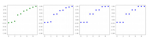
Initial distribution and opinions' evolution of system with (6) at steps 10, 30 and 70;
Initial distribution and opinions' evolution of system with Condition A at steps 20, 40 and 90;
Initial distribution and opinions' evolution for third example at steps 10, 30 and 70, when the equilibrium is reached;