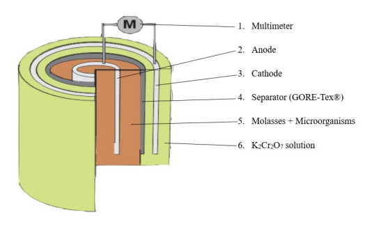
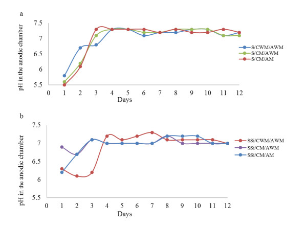
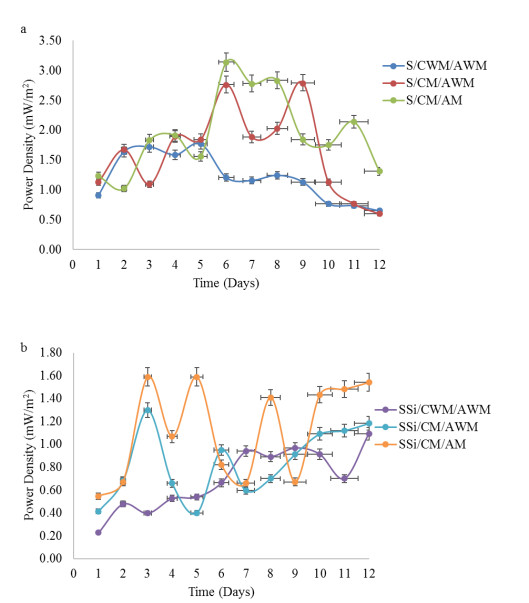
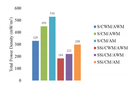
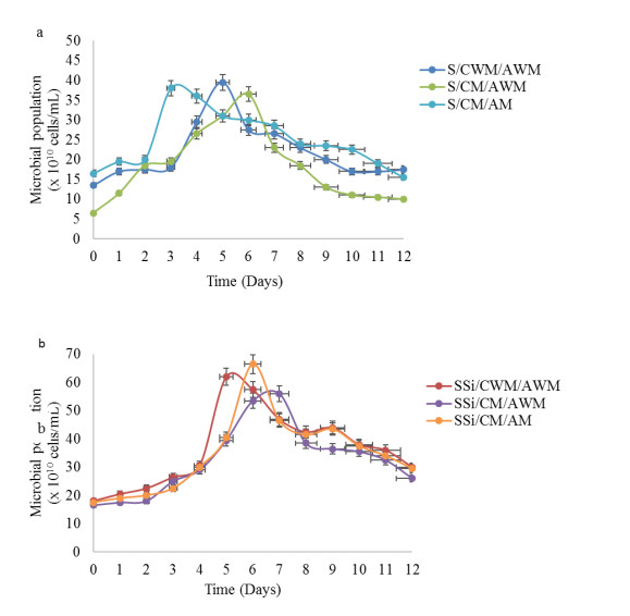
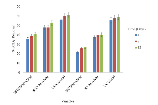
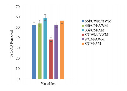
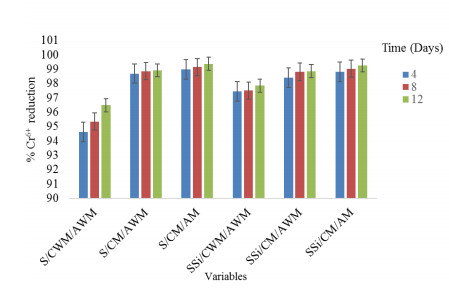
Carcinogenic hexavalent chromium is increasing worldwide due to the increased electroplating, welding and textile industry. On the other hand, molasses, the sugar factory's byproduct with high organic compounds (sugars), may pollute the environment if it is not processed. However, microbial fuel cell (MFC) seems to be a promising technology due to its ability to produce electrical energy from pollutant degradation using microbes while reducing hexavalent chromium to trivalent chromium with less toxicity. Carbon felt was used at both electrodes. This research aimed to determine the effect of modifying the anode with rice bran and cathode with Cu catalyst towards electricity generation and pollutant removal in molasses and reducing Cr (Ⅵ) into Cr (Ⅲ) using tubular microbial fuel cells. Moreover, the effect of mixing Sidoarjo mud and Shewanella oneidensis MR-1 as electricigen bacteria toward electrical energy production and pollutant removal was determined. Experiments revealed that the S/CM/AM variable, which only used Shewanella oneidensis MR-1 as an electricigen bacteria with both modified electrodes, produced the highest total power density of 530.42 mW/m2 and the highest percentage of Cr (Ⅵ) reduction of 98.87%. In contrast, the highest microbial population of 66.5 × 10¹⁰ cells/mL, 61.28% of Biological Oxygen Demand (BOD5) removal and 59.49% of Chemical Oxygen Demand (COD) were achieved by SSi/CM/AM variable, mixing Shewanella oneidensis MR-1 and Sidoarjo mud as an electricigen bacteria with both modified electrodes. Therefore, this study indicates that double chamber tubular microbial fuel cells may be a sustainable solution for managing molasses and carcinogen hexavalent chromium.
Citation: Raden Darmawan, Sri Rachmania Juliastuti, Nuniek Hendrianie, Orchidea Rachmaniah, Nadila Shafira Kusnadi, Ghassani Salsabila Ramadhani, Yawo Serge Marcel, Simpliste Dusabe, Masato Tominaga. Effect of electrode modification on the production of electrical energy and degradation of Cr (Ⅵ) waste using tubular microbial fuel cell[J]. AIMS Environmental Science, 2022, 9(4): 505-525. doi: 10.3934/environsci.2022030
Carcinogenic hexavalent chromium is increasing worldwide due to the increased electroplating, welding and textile industry. On the other hand, molasses, the sugar factory's byproduct with high organic compounds (sugars), may pollute the environment if it is not processed. However, microbial fuel cell (MFC) seems to be a promising technology due to its ability to produce electrical energy from pollutant degradation using microbes while reducing hexavalent chromium to trivalent chromium with less toxicity. Carbon felt was used at both electrodes. This research aimed to determine the effect of modifying the anode with rice bran and cathode with Cu catalyst towards electricity generation and pollutant removal in molasses and reducing Cr (Ⅵ) into Cr (Ⅲ) using tubular microbial fuel cells. Moreover, the effect of mixing Sidoarjo mud and Shewanella oneidensis MR-1 as electricigen bacteria toward electrical energy production and pollutant removal was determined. Experiments revealed that the S/CM/AM variable, which only used Shewanella oneidensis MR-1 as an electricigen bacteria with both modified electrodes, produced the highest total power density of 530.42 mW/m2 and the highest percentage of Cr (Ⅵ) reduction of 98.87%. In contrast, the highest microbial population of 66.5 × 10¹⁰ cells/mL, 61.28% of Biological Oxygen Demand (BOD5) removal and 59.49% of Chemical Oxygen Demand (COD) were achieved by SSi/CM/AM variable, mixing Shewanella oneidensis MR-1 and Sidoarjo mud as an electricigen bacteria with both modified electrodes. Therefore, this study indicates that double chamber tubular microbial fuel cells may be a sustainable solution for managing molasses and carcinogen hexavalent chromium.

| [1] |
Ucal M, Xydis G (2020) Multidirectional relationship between energy resources, climate changes and sustainable development: Technoeconomic analysis. Sustain Cities Soc 60: 102210. https://doi.org/10.1016/j.scs.2020.102210 doi: 10.1016/j.scs.2020.102210

|
| [2] |
Yan JC (2021) The impact of climate policy on fossil fuel consumption: Evidence from the Regional Greenhouse Gas Initiative (RGGI). Energ Econ 100: 105333. https://doi.org/10.1016/j.eneco.2021.105333 doi: 10.1016/j.eneco.2021.105333
|
| [3] |
Lawati MJA, Jafary T, Baawain TMS, et al. (2019) A mini review on biofouling on air cathode of single chamber microbial fuel cell; prevention and mitigation strategies. Biocatal Agric Biotechnol 22: 101370. https://doi.org/10.1016/j.bcab.2019.101370 doi: 10.1016/j.bcab.2019.101370
|
| [4] |
Bist N, Sircar A, Yadav K (2020) Holistic review of hybrid renewable energy in circular economy for valorisation and management. Environ Technol Inno 20: 101054. https://doi.org/10.1016/j.eti.2020.101054 doi: 10.1016/j.eti.2020.101054
|
| [5] |
Gul H, Raza W, Lee J, et al. (2021) Progress in microbial fuel cell technology for wastewater treatment and energy harvesting. Chemosphere 281: 130828. https://doi.org/10.1016/j.chemosphere.2021.130828 doi: 10.1016/j.chemosphere.2021.130828
|
| [6] |
Yaqoob AA, Ibrahim MNM, Rodríguez-Couto S (2020) Development and modification of materials to build cost-effective anodes for microbial fuel cells (MFCs): An overview. Biochem Eng J 164: 107779. https://doi.org/10.1016/j.bej.2020.107779 doi: 10.1016/j.bej.2020.107779
|
| [7] |
Wang HM, Park JD, Ren ZJ (2015) Practical energy harvesting for microbial fuel cells: A review. Environ Sci Technol 49: 3267–3277. https://doi.org/10.1021/es5047765 doi: 10.1021/es5047765
|
| [8] |
Jatoi AS, Akhter F, Mazari SA, et al. (2021) Advanced microbial fuel cell for waste water treatment—a review. Environ Sci Pollut Res 28: 5005–5019. https://doi.org/10.1007/s11356-020-11691-2 doi: 10.1007/s11356-020-11691-2
|
| [9] |
James C, Meenal SH, Elakkiya S, et al. (2020) Sustainable environment through treatment of domestic sewage using MFC. Mater Today: Proc 37: 1495–1502. https://doi.org/10.1016/j.matpr.2020.07.110 doi: 10.1016/j.matpr.2020.07.110
|
| [10] |
Kumar SS, Kumar V, Maylan SK, et al. (2019) Microbial fuel cells (MFCs) for bioelectrochemical treatment of different wastewater streams. Fuel 254: 115526. https://doi.org/10.1016/j.fuel.2019.05.109 doi: 10.1016/j.fuel.2019.05.109
|
| [11] |
Zhou J, Li M, Zhou W, et al. (2020) Efficacy of electrode position in microbial fuel cell for simultaneous Cr(Ⅵ) reduction and bioelectricity production. Sci Total Environ 748: 141425. https://doi.org/10.1016/j.scitotenv.2020.141425 doi: 10.1016/j.scitotenv.2020.141425
|
| [12] |
Sciarria TP, Arioli S, Gargari G, et al. (2019) Monitoring microbial communities' dynamics during the start-up of microbial fuel cells by high-throughput screening techniques. Biotechnol Rep 21: e00310. https://doi.org/10.1016/j.btre.2019.e00310 doi: 10.1016/j.btre.2019.e00310
|
| [13] | Jung SP, Pandit S (2018) Important factors influencing microbial fuel cell performance, In: Mohan SV, Varjani S, Pandey A (Eds.), Biomass, biofuels, biochemicals: Microbial electrochemical technology, chemicals and remediation, Amsterdam: Elsevier, 377–406. https://doi.org/10.1016/B978-0-444-64052-9.00015-7 |
| [14] |
Thygesen A, Poulsen FW, Min B et al. (2009) The effect of different substrates and humic acid on power generation in microbial fuel cell operation. Bioresource Technol 100: 1186–1191. https://doi.org/10.1016/j.biortech.2008.07.067 doi: 10.1016/j.biortech.2008.07.067
|
| [15] |
Hwang JH, Kim KY, Lee WH, et al. (2019) Surfactant addition to enhance bioavailability of bilge water in single chamber microbial fuel cells (MFCs). J Hazard Mater 368: 732–738. https://doi.org/10.1016/j.jhazmat.2019.02.007 doi: 10.1016/j.jhazmat.2019.02.007
|
| [16] |
Bai X, Lin T, Liang N, et al. (2021) Engineering synthetic microbial consortium for efficient conversion of lactate from glucose and xylose to generate electricity. Biochem Eng J 172: 108052. https://doi.org/10.1016/j.bej.2021.108052 doi: 10.1016/j.bej.2021.108052
|
| [17] |
Darmawan R, Widjadja A, Juliastuti SR, et al. (2017) The use of mud as an alternative source for bioelectricity using microbial fuel cells. AIP Conf Proc 1840: 040006. https://doi.org/10.1063/1.4982273 doi: 10.1063/1.4982273
|
| [18] |
Purnomo T, Rachmadiarti F (2018) The changes of environment and aquatic organism biodiversity in east coast of Sidoarjo due to Lapindo hot mud. Int J GEOMATE 15: 181–186. https://doi.org/10.21660/2018.48.IJCST60 doi: 10.21660/2018.48.IJCST60
|
| [19] |
Wang HM, Song XY, Zhang HH, et al. (2020) Removal of hexavalent chromium in dual-chamber microbial fuel cells separated by different ion exchange membranes. J Hazard Mater 384: 121459. https://doi.org/10.1016/j.jhazmat.2019.121459 doi: 10.1016/j.jhazmat.2019.121459
|
| [20] |
GracePavithra K, Jaikumar V, Kumar PS, et al. (2019) A review on cleaner strategies for chromium industrial wastewater: Present research and future perspective. J Clean Prod 228: 580–593. https://doi.org/10.1016/j.jclepro.2019.04.117 doi: 10.1016/j.jclepro.2019.04.117
|
| [21] | Costello RB, Dwyer JT, Merkel JM (2019) Chromium supplements in health and disease, In: Vincent JB (Eds.), The nutritional biochemistry of chromium (Ⅲ), 2 Eds., Amsterdam: Elsevier, 219–249. https://doi.org/10.1016/B978-0-444-64121-2.00007-6 |
| [22] |
Rajaeifar MA, Hemayati SS, Tabatabaei M, et al. (2019) A review on beet sugar industry with a focus on implementation of waste-to-energy strategy for power supply. Renew Sust Energ Rev 103: 423–442. https://doi.org/10.1016/j.rser.2018.12.056 doi: 10.1016/j.rser.2018.12.056
|
| [23] |
Aghbashlo M, Tabatabaei M, Karimi K, et al. (2017) Effect of phosphate concentration on exergetic-based sustainability parameters of glucose fermentation by Ethanolic Mucor indicus. Sustain Prod Consum 9: 28–36. https://doi.org/10.1016/j.spc.2016.06.004 doi: 10.1016/j.spc.2016.06.004
|
| [24] |
Aghbashlo M, Tabatabaei M, Karimi K (2016) Exergy-based sustainability assessment of ethanol production via Mucor indicus from fructose, glucose, sucrose, and molasses. Energy 98: 240–252. https://doi.org/10.1016/j.energy.2016.01.029 doi: 10.1016/j.energy.2016.01.029
|
| [25] |
Xiao N, Wu R, Huang JJ, et al. (2020) Anode surface modification regulates biofilm community population and the performance of micro-MFC based biochemical oxygen demand sensor. Chem Eng Sci 221: 115691. https://doi.org/10.1016/j.ces.2020.115691 doi: 10.1016/j.ces.2020.115691
|
| [26] |
Srivastava P, Yadav AK, Mishra BK (2015) The effects of microbial fuel cell integration into constructed wetland on the performance of constructed wetland. Bioresource Technol 195: 223–230. https://doi.org/10.1016/j.biortech.2015.05.072 doi: 10.1016/j.biortech.2015.05.072
|
| [27] |
Yaqoob AA, Ibrahim MNM, Rafatullah M, et al. (2020) Recent advances in anodes for microbial fuel cells: An overview. Materials 13: 2078. https://doi.org/10.3390/ma13092078 doi: 10.3390/ma13092078
|
| [28] |
Yaqoob AA, Ibrahim MNM, Rodríguez-Couto S (2020) Development and modification of materials to build cost-effective anodes for microbial fuel cells (MFCs): An overview. Biochem Eng J 164: 107779. https://doi.org/10.1016/j.bej.2020.107779 doi: 10.1016/j.bej.2020.107779
|
| [29] |
Liu JH, Ma ZL, Zhu HJ, et al. (2017) Improving xylose utilisation of defatted rice bran for nisin production by overexpression of a xylose transcriptional regulator in Lactococcus lactis. Bioresource Technol 238: 690–697. https://doi.org/10.1016/j.biortech.2017.04.076 doi: 10.1016/j.biortech.2017.04.076
|
| [30] |
Hou TT, Chen N, Tong S, et al. (2019) Enhancement of rice bran as carbon and microbial sources on the nitrate removal from groundwater. Biochem Eng J 148: 185–194. https://doi.org/10.1016/j.bej.2018.07.010 doi: 10.1016/j.bej.2018.07.010
|
| [31] |
Fernandes IJ, Calheiro D, Sánchez FAL, et al. (2017) Characterization of silica produced from rice husk ash: Comparison of purification and processing methods. Mat Res 20: 519–525. http://doi.org/10.1590/1980-5373-MR-2016-1043 doi: 10.1590/1980-5373-MR-2016-1043
|
| [32] | Si FZ, Zang YW, Yan L, et al. (2014) Electrochemical Oxygen Reduction Reaction, In: Xing W, Yin GP, Zhang JJ (Eds.), Rotating electrode methods and oxygen reduction electrocatalysts, Amsterdam: Elsevier, 133–170. https://doi.org/10.1016/B978-0-444-63278-4.00004-5 |
| [33] |
Fan LP, Xu DD, Li C, et al. (2016) Molasses wastewater treatment by microbial fuel cell with MnO2-modified cathode. Pol J Environ Stud 25: 2349–2356. https://doi.org/10.15244/pjoes/64197 doi: 10.15244/pjoes/64197
|
| [34] |
Scott K, Murano C, Rimbu G (2007) A tubular microbial fuel cell. J Appl Electrochem 37: 1063–1068. https://doi.org/10.1007/s10800-007-9355-8 doi: 10.1007/s10800-007-9355-8
|
| [35] |
Flimban SE, Sami GA, Ismail, et al. (2019) Review overview of recent advancements in the microbial fuel cell from fundamentals to applications. Energies 12: 3390. https://doi.org/10.3390/en12173390 doi: 10.3390/en12173390
|
| [36] |
Ye YY, Ngo HH, Guo WS, et al. (2019) Effect of organic loading rate on the recovery of nutrients and energy in a dual-chamber microbial fuel cell. Bioresource Technol 281: 367–373. https://doi.org/10.1016/j.biortech.2019.02.108 doi: 10.1016/j.biortech.2019.02.108
|
| [37] |
Li WW, Sheng GP, Liu XW, et al. (2011) Recent advances in the separators for microbial fuel cells. Bioresource Technol 102: 244–252. https://doi.org/10.1016/j.biortech.2010.03.090 doi: 10.1016/j.biortech.2010.03.090
|
| [38] |
Luo Y, Zhang F, Wei B, et al. (2013) The use of cloth fabric diffusion layers for scalable microbial fuel cells. Biochem Eng J 73: 49–52. https://doi.org/10.1016/j.bej.2013.01.011 doi: 10.1016/j.bej.2013.01.011
|
| [39] |
Zhuang L, Feng CH, Zhou SG (2010) Comparison of membrane- and cloth-cathode assembly for scalable microbial fuel cells: Construction, performance and cost. Process Biochem 45: 929–934. https://doi.org/10.1016/j.procbio.2010.02.014 doi: 10.1016/j.procbio.2010.02.014
|
| [40] | Absher M (1973) Hemocytometer Counting, In: Kruse PK, Pattersom MK (Eds.), Tissue Culture, London: Academic Press, 395–397. |
| [41] |
Muhaimin, Hawa RII, Hidayati ER, et al. (2021) Test method verification of chrome heksavalen (Cr-Ⅵ) test in waste water using UV-visible spectrophotometer. AIP Conf Proc 2370: 030001. https://doi.org/10.1063/5.0062198 doi: 10.1063/5.0062198
|
| [42] |
Wang YJ, Zhao NN, Fang BZ, et al. (2015) Effect of different solvent ratio (ethylene glycol/water) on the preparation of Pt/C catalyst and its activity toward oxygen reduction reaction. RSC Adv 5: 56570–56577. https://doi.org/10.1039/C5RA08068A doi: 10.1039/C5RA08068A
|
| [43] |
Raad NK, Farrokhi F, Mousavi SA, et al. (2020) Simultaneous power generation and sewage sludge stabilisation using an air cathode-MFCs. Biomass Bioenerg 140: 105642. https://doi.org/10.1016/j.biombioe.2020.105642 doi: 10.1016/j.biombioe.2020.105642
|
| [44] |
Tashiro T, Yoshimura F (2019) A neo-logistic model for the growth of bacteria. Physica A 525: 199–215. https://doi.org/10.1016/j.physa.2019.03.049 doi: 10.1016/j.physa.2019.03.049
|
| [45] | Microbial Growth. Bruslind L, 2021. Available from: https://bio.libretexts.org/Bookshelves/Microbiology/Book%3A_Microbiology_(Bruslind)/09%3A_Microbial_Growth. |
| [46] |
Nicola L, Bååth E (2019) The effect of temperature and moisture on lag phase length of bacterial growth in soil after substrate addition. Soil Biol Biochem 137: 107563. https://doi.org/10.1016/j.soilbio.2019.107563 doi: 10.1016/j.soilbio.2019.107563
|
| [47] | Maier RM, Pepper IL (2015) Bacterial growth, In: Pepper IL, Gerba CP, Gentry TJ (Eds.), Environ microbiol, 3 Eds., London: Academic Press: 37–56. https://doi.org/10.1016/B978-0-12-394626-3.00003-X |
| [48] |
Silveira G, Aquino NS, Schneedorf JM (2020) Development, characterisation and application of a low-cost single chamber microbial fuel cell based on hydraulic couplers. Energy 208: 118395. https://doi.org/10.1016/j.energy.2020.118395 doi: 10.1016/j.energy.2020.118395
|
| [49] |
Yarmush M, Pedersen H (1995) Biochemical engineering. Curr Opin Biotech, 6: 189–191. https://doi.org/10.1016/0958-1669(95)80030-1 doi: 10.1016/0958-1669(95)80030-1
|
| [50] |
Nuryana IF, Puspitasari R, Juliastuti SR (2020) Study of electrode modification and microbial concentration for microbial fuel cell effectivity from molasses waste and reduction of heavy metal Cr (Ⅵ) by continue dual chamber reactor. IOP Conf Ser: Mater Sci Eng 823: 012016. https://doi.org/10.1088/1757-899X/823/1/012016 doi: 10.1088/1757-899X/823/1/012016
|
| [51] |
Kaur R, Marwaha A, Chhabra VA, et al. (2020) Recent developments on functional nanomaterial-based electrodes for microbial fuel cells. Renew Sust Energ Rev 119: 109551. https://doi.org/10.1016/j.rser.2019.109551 doi: 10.1016/j.rser.2019.109551
|
| [52] |
Slate AJ, Whitehead KA, Brownson DAC, et al. (2019) Microbial fuel cells: An overview of current technology. Renew Sust Energ Rev 101: 60–81. https://doi.org/10.1016/j.rser.2018.09.044 doi: 10.1016/j.rser.2018.09.044
|
| [53] | Dutta K, Kundu PP (2018) Introduction to microbial fuel cells, In: Progress and recent trends in microbial fuel cells, Amsterdam: Elsevier, 1–6. https://doi.org/10.1016/B978-0-444-64017-8.00001-4 |
| [54] |
Wang G, Huang LP, Zhang YF (2008) Cathodic reduction of hexavalent chromium [Cr(Ⅵ)] coupled with electricity generation in microbial fuel cells. Biotechnol Lett 30: 1959. https://doi.org/10.1007/s10529-008-9792-4 doi: 10.1007/s10529-008-9792-4
|
| [55] |
Lokman NA, Ithnin AM, Yahya WJ, et al. (2021) A brief review on biochemical oxygen demand (BOD) treatment methods for palm oil mill effluents (POME). Environ Technol Inno 21: 101258. https://doi.org/10.1016/j.eti.2020.101258 doi: 10.1016/j.eti.2020.101258
|
| [56] |
Yan FF, Wu C, Cheng YY, et al. (2013) Carbon nanotubes promote Cr(Ⅵ) reduction by alginate-immobilised Shewanella oneidensis MR-1. Biochem Eng J 77: 183–189. https://doi.org/10.1016/j.bej.2013.06.009 doi: 10.1016/j.bej.2013.06.009
|
| [57] |
Aoki Y, Sidiq TP (2014) Ground deformation associated with the eruption of Lumpur Sidoarjo mud volcano, east Java, Indonesia. J Volcanol. Geoth Res 278–279: 96–102. https://doi.org/10.1016/j.jvolgeores.2014.04.012 doi: 10.1016/j.jvolgeores.2014.04.012
|
Figures(13) / Tables(2)

Raden Darmawan, Sri Rachmania Juliastuti, Nuniek Hendrianie, Orchidea Rachmaniah, Nadila Shafira Kusnadi, Ghassani Salsabila Ramadhani, Yawo Serge Marcel, Simpliste Dusabe, Masato Tominaga. Effect of electrode modification on the production of electrical energy and degradation of Cr (Ⅵ) waste using tubular microbial fuel cell[J]. AIMS Environmental Science, 2022, 9(4): 505-525. doi: 10.3934/environsci.2022030


 DownLoad: