An analog electronic circuit model for cAMP-dependent pathway—towards creation of Silicon life

Maria Waqas; Urooj Ainuddin; Umar Iftikhar; Maria Waqas; Urooj Ainuddin; Umar Iftikhar

doi:10.3934/bioeng.2022011

AIMS Bioengineering

2022, Volume 9, Issue 2: 145-162. doi: 10.3934/bioeng.2022011

Previous Article Next Article

Research article

An analog electronic circuit model for cAMP-dependent pathway—towards creation of Silicon life

Department of Computer and Information Systems Engineering, NED University of Engineering and Technology, University Road, Karachi - 75270, Pakistan

Received: 31 January 2022 Revised: 19 March 2022 Accepted: 21 April 2022 Published: 25 April 2022

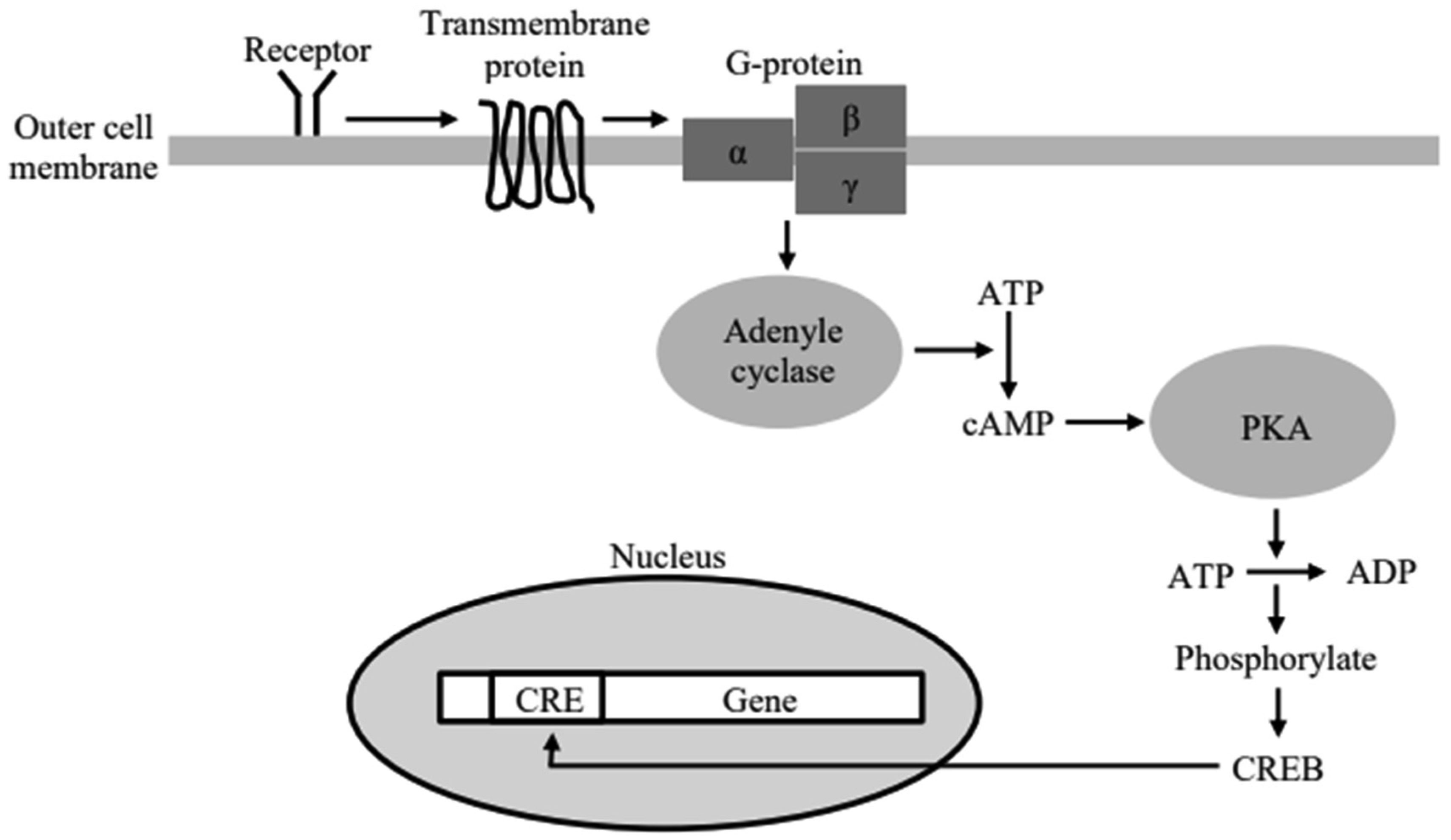
Among the most sought after breakthroughs nowadays to combat computational saturation in the electronic hardware realm, neuromorphic and cytomorphic mimetics of biological structures seem potentially promising. Biological circuits are distinguishable due to their minuscule dimensions and immensely low power consumption; yet they achieve extremely complex and magnificent tasks of life, such as, thinking, memorizing, decision making and self-regulating in response to the surroundings. Low power analog circuit solutions are edged over digital ones as they are inherently noisy and fuzzy like bio-systems. In this paper, an analog circuit equivalent for a well-known biological pathway, cyclic adenosine monophosphate (cAMP), has been proposed, exploiting the fabrication characteristics of an analog transistor. The work demonstrates an application of previously published research of the authors, where it was shown that a single transistor operating in analog mode can mimic some fundamental biological circuit processes like receptor-ligand binding, Michaelis Menten and Hill process reactions. Since biological pathways are chain connections of such reactions, same modular approach can be used to build electronic pathways using those basic transistor circuits. Although the idea of creating silicon life seems far-fetched at this stage, this work supplements the idea of cytomorphic chips which is already gaining interest of bio-engineering community.

Keywords:

Citation: Maria Waqas, Urooj Ainuddin, Umar Iftikhar. An analog electronic circuit model for cAMP-dependent pathway—towards creation of Silicon life[J]. AIMS Bioengineering, 2022, 9(2): 145-162. doi: 10.3934/bioeng.2022011

Related Papers:

[1]	Sheza. M. El-Deeb, Gangadharan Murugusundaramoorthy, Kaliyappan Vijaya, Alhanouf Alburaikan . Certain class of bi-univalent functions defined by quantum calculus operator associated with Faber polynomial. AIMS Mathematics, 2022, 7(2): 2989-3005. doi: 10.3934/math.2022165
[2]	F. Müge Sakar, Arzu Akgül . Based on a family of bi-univalent functions introduced through the Faber polynomial expansions and Noor integral operator. AIMS Mathematics, 2022, 7(4): 5146-5155. doi: 10.3934/math.2022287
[3]	Pinhong Long, Huo Tang, Wenshuai Wang . Functional inequalities for several classes of q-starlike and q-convex type analytic and multivalent functions using a generalized Bernardi integral operator. AIMS Mathematics, 2021, 6(2): 1191-1208. doi: 10.3934/math.2021073
[4]	Erhan Deniz, Hatice Tuǧba Yolcu . Faber polynomial coefficients for meromorphic bi-subordinate functions of complex order. AIMS Mathematics, 2020, 5(1): 640-649. doi: 10.3934/math.2020043
[5]	Shuhai Li, Lina Ma, Huo Tang . Meromorphic harmonic univalent functions related with generalized (p, q)-post quantum calculus operators. AIMS Mathematics, 2021, 6(1): 223-234. doi: 10.3934/math.2021015
[6]	Mohammad Faisal Khan . Certain new applications of Faber polynomial expansion for some new subclasses of $\upsilon$ -fold symmetric bi-univalent functions associated with $q$ -calculus. AIMS Mathematics, 2023, 8(5): 10283-10302. doi: 10.3934/math.2023521
[7]	Khadeejah Rasheed Alhindi, Khalid M. K. Alshammari, Huda Ali Aldweby . Classes of analytic functions involving the q-Ruschweyh operator and q-Bernardi operator. AIMS Mathematics, 2024, 9(11): 33301-33313. doi: 10.3934/math.20241589
[8]	İbrahim Aktaş . On some geometric properties and Hardy class of q-Bessel functions. AIMS Mathematics, 2020, 5(4): 3156-3168. doi: 10.3934/math.2020203
[9]	Ala Amourah, B. A. Frasin, G. Murugusundaramoorthy, Tariq Al-Hawary . Bi-Bazilevič functions of order $\vartheta +i\delta$ associated with $(p, q)-$ Lucas polynomials. AIMS Mathematics, 2021, 6(5): 4296-4305. doi: 10.3934/math.2021254
[10]	Zeya Jia, Nazar Khan, Shahid Khan, Bilal Khan . Faber polynomial coefficients estimates for certain subclasses of $q$ -Mittag-Leffler-Type analytic and bi-univalent functions. AIMS Mathematics, 2022, 7(2): 2512-2528. doi: 10.3934/math.2022141

Abstract

1. Introduction, definitions and preliminaries

In his survey-cum-expository review article, Srivastava ^[35] included also a brief overview of the classical $q$ -analysis versus the so-called $(p, q)$ -analysis with an obviously redundant additional parameter $p$ (see, for details, [,p. 340]). The present sequel to Srivastava's widely-cited review article ^[35], we apply the concept of $q$ -convolution in order to introduce and study the general Taylor-Maclaurin coefficient estimates for functions belonging to a new class of normalized analytic and bi-close-to-convex functions in the open unit disk, which we have defined here.

Let $\mathcal{A}$ denote the class of analytic functions of the form:

$\begin{equation} f(z) = z+\sum\limits_{n = 2}^{\infty}a_{n}\;z^{n} \qquad (z\in \Delta), \end{equation}$

(1.1)

where $\Delta$ denotes the open unit disk in the complex $z$ -plane given by

$\Delta: = \{z: z\in \mathbb{C}\qquad \text{and} \qquad |z| \lt 1\}.$

Also let $\mathcal{S}\subset \mathcal{A}$ consist of functions which are also univalent in $\Delta$ .

If the function $f$ is given by (1.1) and the function $\Upsilon \in \mathcal{A}$ is given by

$\begin{equation} \Upsilon(z) = z+\sum\limits_{n = 2}^{\infty}\psi_{n}z^{n} \qquad (z\in \Delta), \end{equation}$

(1.2)

then the Hadamard product (or convolution) of the functions $f$ and $\Upsilon$ is defined by defined by

$\begin{equation*} (f\ast \Upsilon)(z): = z+\sum\limits_{n = 2}^{\infty}a_{n}\,\psi _{n}\, z^{n} = : (\Upsilon \ast f)(z)\qquad (z\in \Delta). \end{equation*}$

For $0\leqq \alpha < 1,$ we let $S^{\ast}\left(\alpha \right)$ denote the class of functions $g\in \mathcal{S}$ which are starlike of order $\alpha$ in $\Delta$ such that

$\begin{equation*} \Re\left(\frac{zg^{{\prime}}(z)}{g(z)}\right) \gt \alpha \qquad (z\in \Delta). \end{equation*}$

We denote by $\mathcal{C}\left(\alpha \right)$ the class of functions $f\in \mathcal{S}$ which are close-to-convex of order $\alpha$ in $\Delta$ such that (see ^[10,24])

$\begin{equation*} \Re\left(\frac{zf^{\prime}(z)}{g(z)}\right) \gt \alpha \qquad (z \in \Delta), \end{equation*}$

where

$\begin{align*} g\in S^{\ast}\left(0\right) = :S^{\ast}. \end{align*}$

We note that

$S^{\ast}\left(\alpha \right) \subset \mathcal{C}\left( \alpha \right) \subset \mathcal{S}\qquad \text{and} \qquad \left\vert a_{n}\right\vert \lt n \qquad (\forall\; f\in \mathcal{S};\; n\in \mathbb{N}\setminus \{1\})$

by the Bieberbach conjecture or the De Branges Theorem (see ^[3,10]), $\mathbb{N}$ being the set of natural numbers (or the positive integers).

In the above-cited review article, Srivastava ^[35] made use of various operators of $q$ -calculus and fractional $q$ -calculus. We begin by recalling the definitions and notations as follows (see also ^[33] and [45,pp. 350–351]).

The $q$ -shifted factorial is defined, for $\lambda, q\in \mathbb{C}$ and $n \in \mathbb{N}_{0} = \mathbb{N}\cup \{0\}$ , by

$\begin{equation*} (\lambda;q)_{n} = \left\{ \begin{array}{ll} 1 & \qquad (n = 0) \\ \\ \left(1-\lambda \right) \left(1-\lambda q\right) \cdots \left( 1-\lambda q^{n-1}\right) & \qquad (n\in \mathbb{N}). \end{array} \right. \end{equation*}$

By using the $q$ -gamma function $\Gamma_{q}(z),$ we get

$\begin{equation*} \left(q^{\lambda};q\right)_{n} = \frac{\left(1-q\right)^{n}\ \Gamma _{q}\left(\lambda+n\right)}{\Gamma_{q}\left(\lambda \right)} \qquad \left(n\in \mathbb{N}_{0}\right), \end{equation*}$

where (see ^[19,33])

$\begin{equation*} \Gamma_{q}(z) = \left(1-q\right)^{1-z}\;\frac{\left(q;q\right)_{\infty}} {\left(q^{z};q\right)_{\infty}}\qquad \left(\left\vert q\right\vert \lt 1\right) . \end{equation*}$

We note also that

$\begin{equation*} \left(\lambda;q\right)_{\infty } = \prod\limits_{n = 0}^{\infty}\left( 1-\lambda q^{n}\right) \qquad \left(\left\vert q\right\vert \lt 1\right) , \end{equation*}$

and that the $q$ -gamma function $\Gamma_{q}(z)$ satisfies the following recurrence relation:

$\begin{equation*} \Gamma_{q}(z+1) = \left[z\right]_{q}\; \Gamma_{q}(z), \end{equation*}$

where $\left[\lambda\right]_{q}$ denotes the basic (or $q$ -) number defined as follows:

$\begin{equation} \lbrack \lambda]_{q}: = \left\{ \begin{array}{ll} \dfrac{1-q^{\lambda}}{1-q} &\qquad (\lambda\in \mathbb{C})\\ \\ 1+\sum\limits_{j = 1}^{\ell-1}q^{j} &\qquad (\lambda = \ell\in \mathbb{N}). \end{array} \right. \end{equation}$

(1.3)

Using the definition in (1.3), we have the following consequences:

(ⅰ) For any non-negative integer $n\in \mathbb{N}_0$ , the $q$ -shifted factorial is given by

$\begin{equation*} \left[n\right]_{q}!: = \left\{ \begin{array}{ll} 1 & \qquad (n = 0) \\ \\ \prod\limits_{k = 1}^{n}[k]_{q} & \qquad (n\in \mathbb{N}). \end{array} \right. \end{equation*}$

(ⅱ) For any positive number $r$ , the generalized $q$ -Pochhammer symbol is defined by

$\begin{equation*} \left[r\right]_{q,n}: = \left\{ \begin{array}{ll} 1 & \qquad (n = 0)\\ \\ \prod\limits_{k = r}^{r+n-1}[k]_{q} & \qquad (n\in \mathbb{N}). \end{array} \right. \end{equation*}$

In terms of the classical (Euler's) gamma function $\Gamma\left(z\right)$ , it is easily seen that

$\begin{equation*} \lim\limits_{q\rightarrow 1{-}}\{\Gamma_{q}\left(z\right)\} = \Gamma\left(z\right). \end{equation*}$

We also observe that

$\begin{equation*} \lim\limits_{q\rightarrow 1{-}} \left\{\frac{\left(q^{\lambda};q\right) _{n}}{\left(1-q\right)^{n}}\right\} = \left(\lambda \right)_{n}, \end{equation*}$

where $\left(\lambda\right)_{n}$ is the familiar Pochhammer symbol defined by

$\begin{equation*} \left(\lambda \right)_{n} = \left\{ \begin{array}{ll} 1 & \qquad (n = 0) \\ \\ \lambda \left(\lambda +1\right) \cdots \left(\lambda+n-1\right) & \qquad (n\in \mathbb{N}). \end{array} \right. \end{equation*}$

For $0 < q < 1$ , the $q$ -derivative operator (or, equivalently, the $q$ -difference operator) $D_{q}$ is defined by (see ^[22]; see also ^[14,16,21])

$\begin{align*} D_{q}\left(f\ast\Upsilon\right)(z)&\; = D_{q}\left( z+\sum\limits_{n = 2}^{\infty}a_{n}\,\psi_{n}\,z^{n}\right) \\ &: = \frac{\left(f\ast\Upsilon \right)(z) -\left(f\ast\Upsilon \right)(qz)} {z(1-q)} = 1+\sum\limits_{n = 2}^{\infty}[n]_{q}\,a_{n}\, \psi_{n}\,z^{n-1}\qquad (z\in \Delta), \end{align*}$

where, as in the definition (1.3),

$\begin{equation} \left[n\right]_{q} = \left\{ \begin{array}{ll} \dfrac{1-q^{n}}{1-q} = 1+\sum\limits_{j = 1}^{n-1}q^{j}&\qquad (n\in\mathbb{N})\\ \\ 0 &\qquad (n = 0). \end{array} \right. \end{equation}$

(1.4)

Remark 1. Whereas a $q$ -extension of the class of starlike functions was introduced in $1990$ in ^[20] by means of the $q$ -derivative operator $D_q$ , a firm footing of the usage of the $q$ -calculus in the context of Geometric Function Theory was actually provided and the generalized basic (or $q$ -) hypergeometric functions were first used in Geometric Function Theory in an earlier book chapter published in 1989 by Srivastava (see, for details, ^[34]; see also the recent works ^{[25,27,32,36,37,39,40,46,51,52,53,55,56,57]}).

For $\lambda > -1$ and $0 < q < 1$ , El-Deeb et al. ^[14] defined the linear operator $\mathcal{H}_{\Upsilon}^{\lambda, q}:\mathcal{A}\rightarrow \mathcal{A}$ by

$\begin{equation*} \mathcal{H}_{\Upsilon}^{\lambda,q}f(z)\ast\mathcal{M}_{q,\lambda +1}(z) = z\,D_{q}\left(f\ast\Upsilon\right)(z)\qquad (z\in \Delta), \end{equation*}$

where the function $\mathcal{M}_{q, \lambda}(z)$ is given by

$\begin{equation*} \mathcal{M}_{q,\lambda}(z) = z+\sum\limits_{n = 2}^{\infty} \frac{[\lambda]_{q,n-1}}{[n-1]_{q}!}\;z^{n}\qquad (z\in \Delta). \end{equation*}$

A simple computation shows that

$\begin{equation} \mathcal{H}_{\Upsilon}^{\lambda,q}f(z) = z+\sum\limits_{n = 2}^{\infty}\frac{ [n]_{q}!}{[\lambda +1]_{q,n-1}}\;a_{n}\psi_{n}\; z^{n}\qquad (\lambda \gt -1;\; 0 \lt q \lt 1;\; z\in \Delta). \end{equation}$

(1.5)

From the defining relation (1.5), we can easily verify that the following relations hold true for all $f\in \mathcal{A}$ :

$\begin{align} &\text{(i)} \quad [\lambda +1]_{q}\mathcal{H}_{\Upsilon }^{\lambda ,q}f(z) = [\lambda]_{q}\mathcal{H}_{\Upsilon}^{\lambda+1,q}f(z)+q^{\lambda }\,z\ D_{q}\left(\mathcal{H}_{\Upsilon }^{\lambda +1,q}f(z)\right) \qquad (z\in\Delta); \\ &\text{(ii)} \quad \mathcal{I}_{\Upsilon }^{\lambda }f(z): = \lim\limits_{q\rightarrow 1{-}}\mathcal{H}_{\Upsilon}^{\lambda ,q}f(z) = z+\sum\limits_{n = 2}^{\infty}\dfrac{n!}{(\lambda+1)_{n-1}} \,a_{n}\psi_{n}z^{m}\qquad (z\in \Delta). \end{align}$

(1.6)

Remark 2. If we take different particular cases for the coefficients $\psi_{n},$ we obtain the following special cases for the operator $\mathcal{H}_{h}^{\lambda, q}$ :

(ⅰ) For $\psi_{n} = 1$ , we obtain the operator $\mathfrak{J}_{q}^{\lambda}$ defined by Arif et al. ^[2] as follows (see also Srivastava ^[47]):

$\begin{equation} \mathfrak{J}_{q}^{\lambda}f(z) : = z+\sum\limits_{n = 2}^{\infty}\frac{[n]_{q}!} {[\lambda+1]_{q,n-1}}\;a_{n}\,z^{n}\qquad (z\in \Delta); \end{equation}$

(1.7)

(ⅱ) For

$\psi_{n} = \dfrac{(-1)^{n-1}\;\Gamma(\upsilon+1)}{ 4^{n-1}\; (n-1)! \;\Gamma(n+\upsilon)} \qquad \text{and} \qquad \upsilon \gt 0,$

we obtain the operator $\mathcal{N}_{\upsilon, q}^{\lambda}$ defined by El-Deeb and Bulboacǎ ^[12] and El-Deeb ^[11] as follows (see also ^[16]):

$\begin{align} \mathcal{N}_{\upsilon,q}^{\lambda}f(z)&: = z+\sum\limits_{n = 2}^{\infty}\frac{ (-1)^{n-1}\Gamma(\upsilon+1)}{4^{n-1}\; (n-1)! \;\Gamma(n+\upsilon)}\cdot \frac{[n]_{q}!}{[\lambda +1]_{q,n-1}}\;a_{n}\,z^{n} \\ &\; = z+\sum\limits_{n = 2}^{\infty}\frac{[n]_{q}!}{[\lambda+1]_{q,n-1}}\;\phi _{n}\,a_{n}\,z^{n} \end{align}$

(1.8)

$(\upsilon \gt 0;\;\lambda \gt -1;\;0 \lt q \lt 1;\ z\in \Delta),$

where

$\begin{equation} \phi_{n}: = \frac{(-1)^{n-1}\;\Gamma(\upsilon+1)}{4^{n-1}\; (n-1)! \;\Gamma (n+\upsilon)} \qquad (n \in \mathbb{N}\setminus\{1\}); \end{equation}$

(1.9)

(ⅲ) For

$\psi_{n} = \left(\dfrac{n+1}{m+n}\right)^{\alpha}, \quad \alpha \gt 0 \qquad \text{and} \qquad n \in \mathbb{N}_0,$

we obtain the operator $\mathcal{M}_{m, q}^{\lambda, \alpha}$ defined by El-Deeb and Bulboacǎ (see ^[13,43]) as follows:

$\begin{equation} \mathcal{M}_{m,q}^{\lambda,\alpha}f(z): = z+\sum\limits_{n = 2}^{\infty }\left(\frac{m+1}{m+n}\right)^{\alpha}\cdot \frac{[n]_{q}!} {[\lambda+1]_{q,n-1}}\;a_{n}\, z^{n}\qquad (z\in \Delta) ; \end{equation}$

(1.10)

(ⅳ) For

$\psi_{n} = \dfrac{\rho^{n-1}}{(n-1)!}\;e^{-\rho} \qquad \text{and} \qquad \rho \gt 0,$

we obtain a $q$ -analogue of the Poisson operator defined in ^[30] by

$\begin{equation} \mathcal{I}_{q}^{\lambda,\rho}f(z): = z+\sum\limits_{n = 2}^{\infty}\frac{ \rho^{n-1}}{(n-1)!}\;e^{-\rho}\cdot \frac{[n]_{q}!}{[\lambda +1]_{q,n-1}}\; a_{n}\,z^{n}\qquad (z\in \Delta); \end{equation}$

(1.11)

(ⅴ) For

$\psi_{n} = \binom{m+n-2}{n-1}\; \theta^{n-1}\left(1-\theta \right)^{m}\qquad \left(m\in \mathbb{N};\; 0\leqq \theta \leqq 1\right),$

we get a $q$ -analogue $\Psi_{q, \theta}^{\lambda, m}$ of the Pascal distribution operator as follows (see ^[15]):

$\begin{equation} \Psi_{q,\theta}^{\lambda,m}f(z): = z+\sum\limits_{n = 2}^{\infty} \binom{m+n-2}{n-1}\theta^{n-1}\left(1-\theta \right)^{m}\cdot \frac{[n]_{q}!}{[\lambda+1]_{q,n-1}}\;a_{n}\; z^{n} \end{equation}$

(1.12)

$(z\in \Delta).$

If $f$ and $F$ are analytic functions in $\Delta$ , we say that the function $f$ is subordinate to the function $F$ , written as $f(z)\prec F(z)$ , if there exists a Schwarz function $s$ , which is analytic in $\Delta$ with $s(0) = 0$ and $\left\vert s(z)\right\vert < 1$ for all $z\in \Delta$ , such that

$f(z) = F\big(s(z)\big) \qquad (z\in \Delta).$

Furthermore, if the function $F$ is univalent in $\Delta$ , then we have the following equivalence (see, for example, ^[7,28])

$\begin{equation*} f(z)\prec F(z)\; \Longleftrightarrow \; f(0) = F(0)\qquad \text{and} \qquad f(\Delta)\subset F(\Delta). \end{equation*}$

The Koebe one-quarter theorem (see ^[10]) asserts that the image of $\Delta$ under every univalent function $f\in \mathcal{S}$ contains the disk of radius $\dfrac{1}{4}$ . Therefore, every function $f\in \mathcal{S}$ has an inverse $f^{-1}$ which satisfies the following inequality:

$\begin{equation*} f\big(f^{-1}(w)\big) = w\qquad \left(\left\vert w\right\vert \lt r_{0}\left(f\right); \;r_{0}\left(f\right) \geqq \frac{1}{4}\right) , \end{equation*}$

where

$\begin{align*} g(w) & = f^{-1}(w) = w-a_{2}w^{2}+\left(2a_{2}^{2}-a_{3}\right) w^{3}-\left( 5a_{2}^{3}-5a_{2}a_{3}+a_{4}\right) w^{4}+\cdots \\ & = w+\sum\limits_{n = 2}^{\infty}A_{n}\; w^{n}. \end{align*}$

A function $f\in \mathcal{A}$ is said to be bi-univalent in $\Delta$ if both $f$ and $f^{-1}$ are univalent in $\Delta$ . Let $\Sigma$ denote the class of normalized analytic and bi-univalent functions in $\Delta$ given by (1.1). The class $\Sigma$ of analytic and bi-univalent functions was introduced by Lewin ^[26], where it was shown that

$f\in \Sigma \;\Longrightarrow\;\left\vert a_{2}\right\vert \lt 1.51.$

Brannan and Clunie ^[4] improved Lewin's result to the following form:

$f\in \Sigma \;\Longrightarrow\; \left\vert a_{2}\right\vert \lt \sqrt{2}$

and, subsequently, Netanyahu ^[29] proved that

$f\in \Sigma \;\Longrightarrow\;\left\vert a_{2}\right\vert \lt \frac{4}{3}.$

It should be noted that the following functions:

$f_{1}(z) = \dfrac{z}{1-z},\quad f_{2}(z) = \dfrac{1}{2}\log\left(\dfrac{1+z}{1-z}\right) \qquad \text{and} \qquad f_{3}(z) = -\log (1-z),$

together with their corresponding inverses given by

$f_{1}^{-1}(w) = \dfrac{w}{1+w}, \quad f_{2}^{-1}(w) = \dfrac{e^{2w}-1}{e^{2w}+1} \qquad \text{and} \qquad f_{3}^{-1}(w) = \dfrac{e^{w}-1}{e^{w}},$

are elements of the analytic and bi-univalent function class $\Sigma$ (see ^[14,48]). A brief history and interesting examples of the analytic and bi-univalent function class $\Sigma$ can be found in (for example) ^[5,48].

Brannan and Taha ^[6] (see also ^[48]) introduced certain subclasses of the bi-univalent function class $\Sigma$ similar to the familiar subclasses $S^{\ast }\left(\alpha \right)$ and $K\left(\alpha \right)$ of starlike and convex functions of order $\alpha \; \left(0\leqq \alpha < 1\right)$ , respectively (see ^[5]). Indeed, following Brannan and Taha ^[6], a function $f\in \mathcal{A}$ is said to be in the class $S_{\Sigma}^{\ast }\left(\alpha \right)$ of bi-starlike functions of order $\alpha \; \left(0 < \alpha \leqq 1\right)$ , if each of the following conditions is satisfied:

$\begin{equation*} f\in \Sigma \qquad \text{and}\qquad \left\vert \arg\left(\frac{zf^{\prime}(z)}{ f(z)}\right)\right\vert \lt \frac{\alpha \pi}{2}\qquad (z\in \Delta) \end{equation*}$

and

$\begin{equation*} \left\vert \arg\left(\frac{z\mathcal{F}^{\prime}(w)}{\mathcal{F}(w)}\right\vert\right) \lt \frac{\alpha \pi }{2} \qquad (w\in \Delta), \end{equation*}$

where the function $\mathcal{F}$ is the analytic extension of $f^{-1}$ to $\Delta$ , given by

$\begin{equation} \mathcal{F}(w) = w-a_{2}w^{2}+\left( 2a_{2}^{2}-a_{3}\right) w^{3}-\left( 5a_{2}^{3}-5a_{2}a_{3}+a_{4}\right) w^{4}+\cdots \qquad (w\in \Delta). \end{equation}$

(1.13)

A function $f\in A$ is said to be in the class $K_{\Sigma}^{\ast }\left(\alpha \right)$ of bi-convex functions of order $\alpha \; \left(0 < \alpha \leqq 1\right)$ , if each of the following conditions is satisfied:

$\begin{equation*} f\in \Sigma ,\quad \text{with}\quad \left\vert \arg\left(1+\frac{ zf^{\prime \prime }(z)}{f^{\prime}(z)}\right) \right\vert \lt \frac{\alpha \pi }{2} \qquad (z\in \Delta) \end{equation*}$

and

$\begin{equation*} \left\vert \arg\left(1+\frac{zg^{\prime \prime}(w)}{g^{\prime}(w)} \right) \right\vert \lt \frac{\alpha \pi }{2}\qquad (w\in \Delta). \end{equation*}$

The classes $S_{\Sigma}^{\ast}\left(\alpha \right)$ and $K_{\Sigma}\left(\alpha \right)$ of bi-starlike functions of order $\alpha$ in $\Delta$ and bi-convex functions of order $\alpha \; \left(0 < \alpha \leqq 1\right)$ in $\Delta$ , corresponding to the function classes $S^{\ast}\left(\alpha \right)$ and $K\left(\alpha \right)$ , were also introduced analogously. For each of the function classes $S_{\Sigma}^{\ast}\left(\alpha \right)$ and $K_{\Sigma}\left(\alpha \right)$ , non-sharp estimates on the first two Taylor-Maclaurin coefficients $\left\vert a_{2}\right\vert$ and $\left\vert a_{3}\right\vert$ are known (see ^[6,35,48]). In fact, this pioneering work by Srivastava et al. ^[48] happens to be one of the most important studies of the bi-univalent function class $\Sigma$ . It not only revived the study of the bi-univalent function class $\Sigma$ in recent years, but it has also inspired remarkably many investigations in this area including the present paper. Some of these many recent papers dealing with problems involving the analytic and bi-univalent functions such as those considered in this article include ^{[1,9,17,23,48]}, and indeed also many other works (see, for example, ^[38,44,54]).

Sakar and Güney ^[31] introduced and studied the following class:

$\mathcal{T}_{\Sigma}\left( \lambda,\beta \right) \;\; \left(0\leqq \lambda \leqq 1;\; 0\leqq \beta \lt 1\right).$

In the same way, we define the following subclass of bi-close-to-convex functions $\mathcal{H}_{\Sigma}^{q, \lambda }\left(\eta, \beta, \Upsilon \right)$ as follows.

Definition 1. For $0\leqq \eta < 1$ and $0\leqq \beta \leqq 1, \;$ a function $f\in \Sigma$ has the form (1.1) and the function $\Upsilon$ given by (1.2), the function $f$ is said to be in the class $\mathcal{H}_{\Sigma}^{q, \lambda}\left(\eta, \beta, \Upsilon\right)$ if there exists a function $g \in \mathcal{S}^{\ast}$ such that

$\begin{equation} \Re\left(\frac{z\left(\mathcal{H}_{\Upsilon}^{\lambda ,q}f(z)\right) ^{{\prime }}+\beta z^{2}\left( \mathcal{H}_{\Upsilon }^{\lambda ,q}f(z)\right)^{\prime\prime}}{\left(1-\beta \right) \mathcal{H}_{\Upsilon }^{\lambda,q}g(z)+\beta z\left(\mathcal{H}_{\Upsilon }^{\lambda,q}g(z)\right)^{\prime}}\right) \gt \eta \qquad (z\in \Delta) \end{equation}$

(1.14)

and

$\begin{equation} \Re\left(\frac{z\left(\mathcal{H}_{\Upsilon}^{\lambda,q}\mathcal{F }(w)\right)^{{\prime}}+\beta z^{2}\left(\mathcal{H}_{\Upsilon}^{\lambda ,q}\mathcal{F}(w)\right) ^{^{{\prime \prime }}}}{\left(1-\beta \right) \mathcal{H}_{\Upsilon }^{\lambda,q}\mathcal{G}(w)+\beta z\left(\mathcal{H} _{\Upsilon }^{\lambda ,q}\mathcal{G}(w)\right)^{{\prime}}}\right) \gt \eta \qquad (w\in \Delta), \end{equation}$

(1.15)

where the function $\mathcal{F}$ is the analytic extension of $f^{-1}$ to $\Delta$ , and is given by (1.13), and $\mathcal{G}$ is the analytic extension of $g^{-1}$ to $\Delta$ as follows:

$\begin{equation} \mathcal{G}(w) = w-b_{2}w^{2}+\left(2b_{2}^{2}-b_{3}\right)w^{3}-\left( 5b_{2}^{3}-5b_{2}b_{3}+b_{4}\right) w^{4}+\cdots \qquad (w\in \Delta). \end{equation}$

(1.16)

We note that, if $b_{n} = a_{n}\; \; (n\in \mathbb{N}\setminus\{1\})$ , $\mathcal{S}_{\Sigma }^{q, \lambda}\left(\eta, \beta, \Upsilon\right)$ becomes the class of bi-starlike functions satisfying the following inequalities:

$\begin{equation} \Re\left(\frac{z\left(\mathcal{H}_{\Upsilon}^{\lambda ,q}f(z)\right)^{{\prime}}+\beta z^{2}\left(\mathcal{H}_{\Upsilon }^{\lambda ,q}f(z)\right) ^{\prime \prime}}{\left( 1-\beta \right) \mathcal{H}_{\Upsilon }^{\lambda ,q}f(z)+\beta z\left( \mathcal{H}_{\Upsilon }^{\lambda ,q}f(z)\right)^{\prime}}\right) \gt \eta \qquad (z\in \Delta). \end{equation}$

(1.17)

and

$\begin{equation} \Re\left(\frac{z\left(\mathcal{H}_{\Upsilon}^{\lambda ,q}\mathcal{F }(w)\right) ^{{\prime}}+\beta z^{2}\left(\mathcal{H}_{\Upsilon}^{\lambda ,q}\mathcal{F}(w)\right)^{\prime \prime}}{\left(1-\beta \right) \mathcal{H}_{\Upsilon}^{\lambda,q}\mathcal{F}(w)+\beta z\left( \mathcal{H} _{\Upsilon }^{\lambda ,q}\mathcal{F}(w)\right)^{\prime}}\right) \gt \eta \qquad (w\in \Delta). \end{equation}$

(1.18)

Remark 3. Each of the following limit cases when $q\rightarrow 1{-}$ is worthy of note.

(ⅰ) Putting $q\rightarrow 1{-}$ , we obtain

$\lim\limits_{q\rightarrow 1{-}}\mathcal{H}_{\Sigma }^{q,\lambda}\left(\eta,\beta,h\right) = : \mathcal{P}_{\Sigma}^{\lambda}\left(\eta,\beta,h\right),$

where $\mathcal{P}_{\Sigma}^{\lambda }\left(\eta, \beta, \Upsilon \right)$ represents the functions $f\in \Sigma$ that satisfy (1.14) and (1.15) with $\mathcal{H}_{\Upsilon}^{\lambda, q}$ replaced by $\mathcal{I}_{\Upsilon}^{\lambda}$ as in (1.6).

(ⅱ) Putting

$\psi_{n} = \dfrac{(-1)^{n-1}\Gamma(\upsilon+1)}{ 4^{n-1}\; (n-1)! \;\Gamma(m+\upsilon)}\qquad (\upsilon \gt 0),$

we obtain the class $\mathcal{B}_{\Sigma}^{q, \lambda} \left(\eta, \beta, \upsilon\right)$ representing the functions $f\in \Sigma$ that satisfy (1.14) and (1.15) with $\mathcal{H}_{\Upsilon}^{\lambda, q}$ replaced by $\mathcal{N}_{\upsilon, q}^{\lambda}$ as in (1.8).

(ⅲ) Putting

$\psi_{n} = \left(\dfrac{n+1}{m+n}\right)^{\alpha}\qquad (\alpha \gt 0;\; m\geqq \mathbb{N}_0),$

we obtain the class $\mathcal{L}_{\Sigma}^{\lambda, q} \left(\eta, \beta, m, \alpha \right)$ consisting of the functions $f\in \Sigma$ that satisfy (1.14) and (1.15) with $\mathcal{H} _{\Upsilon}^{\lambda, q}$ replaced by $\mathcal{M}_{m, q}^{\lambda, \alpha }$ as in (1.10).

(ⅳ) Putting

$\psi_{n} = \dfrac{\rho^{n-1}}{(n-1)!}\;e^{-\rho }\qquad (\rho \gt 0),$

we obtain the class $\mathcal{M}_{\Sigma}^{q, \lambda}\left(\eta, \beta, \rho \right)$ representing the functions $f\in \Sigma$ which satisfy the inequalities in (1.14) and (1.15) with $\mathcal{H}_{\Upsilon}^{\lambda, q}$ replaced by $\mathcal{I}_{q}^{\lambda, \rho}$ as in (1.11).

(ⅴ) Putting

$\psi_{n} = \binom{m+n-2}{n-1}\; \theta^{n-1}\left(1-\theta \right)^{m}\qquad \left(m\in \mathbb{N};\; 0\leqq \theta \leqq 1\right),$

we get the class $\mathcal{W}_{\Sigma}^{q, \lambda}\left(\eta, \beta, m, \theta \right)$ of the functions $f\in \Sigma$ which satisfy the inequalities in (1.14) and (1.15) with $\mathcal{H}_{\Upsilon}^{\lambda, q}$ replaced by $\Psi_{q, \theta}^{\lambda, m}$ occurring in (1.12).

Using the Faber polynomial expansion of functions $f\in \mathcal{A}$ which have the normalized form (1.1), the coefficients of its inverse map may be expressed as follows (see ^[18]):

$\begin{equation} \mathcal{F}(w) = f^{-1}(w) = w+\sum\limits_{n = 2}^{\infty}\frac{1}{n}\; K_{n-1}^{-n}(a_{2},a_{3},\cdots)\;w^{n} = w+\sum\limits_{n = 2}^{\infty}A_{n}\;w^{n}, \end{equation}$

(1.19)

where

$\begin{align} \mathcal{K}_{n-1}^{-n}(a_{2},a_{3},\cdots) & = \frac{(-n)!}{(-2n+1)!\; (n-1)!} a_{2}^{n-1} \\ &\qquad +\frac{(-n)!}{(2(-n+1))!\; (n-3)!}\;a_{2}^{n-3}\;a_{3} \\ &\qquad +\frac{(-n)!}{(-2n+3)!\; (n-4)!}\;a_{2}^{n-4}\;a_{4} \\ &\qquad +\frac{(-n)!}{ (2(-n+2))!\; (n-5)!}\;a_{2}^{n-5}\;\left[a_{5}+\left(-n+2\right)a_{3}^{2}\right] \\ &\qquad +\frac{(-n)!}{(-2n+5)!\; (n-6)!}\;a_{2}^{n-6} \left[a_{6}+\left(-2n+5\right) a_{3}\;a_{4}\right] \\ &\qquad +\sum\limits_{j\geqq 7}a_{2}^{n-j}U_{j} \end{align}$

(1.20)

such that $U_{j}$ with $7\leqq j\leqq n$ is a homogeneous polynomial in the variables $a_{2}, a_{3}, \cdots, a_{n}$ . Here such expressions as (for example) $(-n)!$ are to be interpreted symbolically by

$\begin{equation*} (-n)!\equiv \Gamma(1-n): = (-n)(-n-1)(-n-2)\cdots \qquad \big(n\in \mathbb{N}_0\big). \end{equation*}$

In particular, the first three terms of $\mathcal{K}_{n-1}^{-n}$ are given by

$\begin{align*} \mathcal{K}_{1}^{-2} = -2a_{2}, \end{align*}$

$\begin{align*} \mathcal{K}_{2}^{-3} = 3\left(2a_{2}^{2}-a_{3}\right) \end{align*}$

and

$\begin{align*} \mathcal{K}_{3}^{-4} = -4\left(5a_{2}^{3}-5a_{2}a_{3}+a_{4}\right). \end{align*}$

In general, an expansion of $\mathcal{K}_{m}^{-n} \; (n\in \mathbb{N})$ is given by (see ^{[1,8,41,42,47,49,50]})

$\begin{equation*} \mathcal{K}_{m}^{-n} = na_{m}+\frac{n\left(n-1\right)}{2}\;\mathcal{D}_{m}^{2}+ \frac{n!}{3!\;\left(n-3\right)!}\;\mathcal{D}_{m}^{3}+\cdots+\frac{n!}{m!\left( n-m\right)!}\;\mathcal{D}_{m}^{m}, \end{equation*}$

where

$\mathcal{D}_{m}^{n} = \mathcal{D}_{m}^{n}(a_{2},a_{3},a_{4},\cdots)$

and, alternatively,

$\begin{equation*} \mathcal{D}_{m}^{n}(a_{2},a_{3},\cdots,a_{m+1}) = \sum\limits_{i_1,\cdots,i_m}\left(\frac{n!}{ i_{1}!\;\cdots\; i_{m}!}\right)\;a_{2}^{i_{1}}\;\cdots\; a_{m+1}^{i_{m}}, \end{equation*}$

where $a_{1} = 1$ and the sum is taken over all non-negative integers $i_{1}, \cdots, i_{m}$ satisfying the following constraints:

$i_{1}+i_{2}+\cdots+i_{m} = n$

and

$i_{1}+2i_{2}+\cdots+mi_{m} = m.$

Evidently, we have

$\begin{equation*} \mathcal{D}_{m}^{m}(a_{2},a_{3},\cdots,a_{m+1}) = a_{2}^{m}. \end{equation*}$

The following Lemma will be needed to prove our results.

The Carathéodory Lemma. (see ^[10]) If $\phi \in \mathfrak{P}$ and

$\phi(z) = 1+\sum\limits_{n = 1}^{\infty}c_{n}\;z^{n},$

then

$|c_{n}|\leqq 2 \qquad (n \in \mathbb{N}).$

This inequality is sharp for all positive integers $n$ . Here $\mathfrak{P}$ is the family of all functions $\phi,$ which analytic and have positive real part in $\Delta,$ with $\phi(0) = 1$ .

2. A set of main results

In this section, we apply the above-described Faber polynomial expansion method, we derive bounds for the general Taylor-Maclaurin coefficients of functions in $\mathcal{H}_{\Sigma}^{q, \lambda}\left(\eta, \beta, \Upsilon \right)$ .

Theorem 1. Let the function $f$ given by (1.1) belong to the class $\mathcal{H}_{\Sigma}^{q, \lambda}\left(\eta, \beta, \Upsilon \right)$ . Suppose also that

$0\leqq \eta \lt 1,\quad 0\leqq \beta \leqq 1,\quad \lambda \gt -1 \qquad \mathit{\text{and}} \qquad 0 \lt q \lt 1.$

If $a_{k} = 0$ for $2\leqq k\leqq n-1,$ then

$\begin{equation*} \left\vert a_{n}\right\vert \leqq \frac{2\left(1-\eta \right) [\lambda +1]_{q,n-1}}{n\left[1+\left(n-1\right)\beta\right] \ [n]_{q}!\,\psi _{n}} +1. \end{equation*}$

Proof. If $f\in \mathcal{H}_{\Sigma }^{q, \lambda }\left(\eta, \beta, \Upsilon \right)$ , then there exists a function $g(z)$ , given by

$g(z): = z+\sum\limits_{n = 2}^{\infty}b_{n}\;z^{n}\in S^{\ast},$

such that

$\begin{equation*} \Re\left(\frac{z\left(\mathcal{H}_{\Upsilon}^{\lambda ,q}f(z)\right)^{\prime}+\beta z^{2}\left( \mathcal{H}_{\Upsilon }^{\lambda ,q}f(z)\right)^{\prime \prime}}{\left(1-\beta \right) \mathcal{H}_{\Upsilon}^{\lambda,q}g(z)+\beta z\left(\mathcal{H}_{\Upsilon }^{\lambda,q}g(z)\right)^{{\prime}}}\right) \gt \eta \qquad (z\in \Delta). \end{equation*}$

Moreover, by using the Faber polynomial expansion, we have

$\begin{align} &\frac{z\left(\mathcal{H}_{\Upsilon }^{\lambda,q}f(z)\right)^{\prime} +\beta z^{2}\left(\mathcal{H}_{\Upsilon}^{\lambda ,q}f(z)\right) ^{\prime \prime}}{\left(1-\beta \right) \mathcal{H}_{\Upsilon }^{\lambda ,q}g(z)+\beta z\left(\mathcal{H}_{\Upsilon }^{\lambda ,q}g(z)\right)^{\prime}} \\ &\qquad = 1+\sum\limits_{n = 2}^{\infty}\Bigg(\left[1+\beta \left(n-1\right) \right]\; \frac{[n]_{q}!}{[\lambda+1]_{q,n-1}}\,\psi _{n}\left(na_{n}-b_{n}\right) \\ &\qquad \qquad \qquad +\sum\limits_{t = 1}^{n-2}\dfrac{[n,q]!} {[\lambda +1,q]_{n-1}}\,\psi _{n}\left[1+\left(n-t-1\right)\beta \right] \\ &\qquad \qquad \qquad \qquad \cdot K_{t}^{-1}\left[\left( 1+\beta \right) b_{2},\left(1+2\beta \right) b_{3},\cdots, \left(1+t\beta \right) b_{t+1}\right] \\ &\qquad \qquad \qquad \qquad \cdot \left[\left(n-t\right)\ a_{n-t}-b_{n-t}\right] \Bigg) z^{n-1}\qquad (z\in \Delta). \end{align}$

(2.1)

Also, for the inverse map $\mathcal{F} = f^{-1},$ there exists a function $\mathcal{G}(w)$ , given by

$\mathcal{G}(w) = w+\sum\limits_{n = 2}^{\infty}B_{n}\;w^{n}\in S^{\ast},$

such that

$\begin{equation*} \Re\left(\frac{z\left( \mathcal{H}_{\Upsilon }^{\lambda ,q}\mathcal{F }(w)\right) ^{{\prime }}+\beta z^{2}\left( \mathcal{H}_{\Upsilon }^{\lambda ,q}\mathcal{F}(w)\right) ^{{{\prime \prime }}}}{\left( 1-\beta \right) \mathcal{H}_{\Upsilon }^{\lambda ,q}\mathcal{G}(w)+\beta z\left( \mathcal{H} _{\Upsilon }^{\lambda ,q}\mathcal{G}(w)\right) ^{{\prime }}}\right) \gt \eta \qquad (w\in \Delta), \end{equation*}$

the Faber polynomial expansion of the inverse map $\mathcal{F} = f^{-1}$ is given by

$\mathcal{F}(w) = w+\sum\limits_{n = 2}^{\infty}A_{n}\;w^{n},$

so we have

$\begin{align} &\frac{z\left(\mathcal{H}_{\Upsilon}^{\lambda,q}\mathcal{F}(w)\right) ^{\prime}+\beta z^{2}\left(\mathcal{H}_{\Upsilon}^{\lambda,q}\mathcal{ F}(w)\right)^{\prime \prime}}{\left(1-\beta \right) \mathcal{H} _{\Upsilon }^{\lambda ,q}\mathcal{G}(w)+\beta z\left(\mathcal{H}_{\Upsilon }^{\lambda ,q}\mathcal{G}(w)\right)^{\prime}} \\ &\qquad = 1+\sum\limits_{n = 2}^{\infty}\Bigg(\left[1+\beta \left(n-1\right)\right]\;\frac{[n]_{q}!}{[\lambda +1]_{q,n-1}}\,\psi _{n}\left(nA_{n}-B_{n}\right) \\ &\qquad \qquad +\sum\limits_{t = 1}^{n-2}\frac{[n]_{q}!}{[\lambda +1]_{q,n-1}}\psi _{n}\left[1+\left(n-t-1\right) \beta \right] \\ &\qquad \qquad \qquad \cdot K_{t}^{-1}\left[\left( 1+\beta \right) B_{2},\left( 1+2\beta \right) B_{3},\cdots,\left(1+t\beta \right) B_{t+1}\right] \\ &\qquad \qquad \qquad \cdot \left[\left(n-t\right) A_{n-t}-B_{n-t}\right] \Bigg)\; w^{n-1}\qquad (w\in \Delta). \end{align}$

(2.2)

Now, since

$\begin{equation*} f\in \mathcal{H}_{\Sigma}^{q,\lambda}\left(\eta,\beta,\Upsilon \right) \qquad \text{and}\qquad \mathcal{F} = f^{-1}\in \mathcal{H}_{\Sigma}^{q,\lambda }\left(\eta,\beta,\Upsilon \right) , \end{equation*}$

there are the following two positive real part functions:

$\begin{equation*} U(z) = 1+\sum\limits_{n = 1}^{\infty}c_{n}\;z^{n} \end{equation*}$

and

$\begin{equation*} V(w) = 1+\sum\limits_{n = 1}^{\infty}d_{n}\;w^{n}, \end{equation*}$

for which

$\begin{equation*} \Re\big(U(z)\big) \gt 0\qquad \text{and} \qquad \Re\big( V(w)\big) \gt 0 \qquad (z,w\in \Delta), \end{equation*}$

so that

(2.3)

and

$\begin{align} &\frac{z\left(\mathcal{H}_{\Upsilon }^{\lambda ,q}\mathcal{F}(w)\right) ^{{\prime }}+\beta z^{2}\left(\mathcal{H}_{\Upsilon }^{\lambda ,q}\mathcal{ F}(w)\right)^{\prime \prime}}{\left(1-\beta \right) \mathcal{H} _{\Upsilon }^{\lambda ,q}\mathcal{G}(w)+\beta z\left(\mathcal{H}_{\Upsilon }^{\lambda ,q}\mathcal{G}(w)\right)^{\prime}} = \eta +\left(1-\eta \right)\; V(w) \\ &\qquad = 1+\left(1-\eta \right)\sum\limits_{n = 1}^{\infty}d_{n}\;w^{n}. \end{align}$

(2.4)

Now, under the assumption that $a_{k} = 0$ for $0\leqq k\leqq n-1,$ we obtain $A_{n} = -a_{n}.$ Then, by using (2.1) and comparing the corresponding coefficients in (2.3), we obtain

$\begin{equation} \left[1+\beta \left(n-1\right)\right] \;\frac{[n]_{q}!}{[\lambda+1]_{q,n-1} }\,\psi_{n}\left(na_{n}-b_{n}\right) = \left(1-\eta \right)\; c_{n-1}. \end{equation}$

(2.5)

Similarly, by using (2.2) in the Eq (2.4), we find that

$\begin{equation} \left[1+\beta \left(n-1\right) \right]\; \frac{[n]_{q}!}{[\lambda +1]_{q,n-1} }\,\psi_{n}\left(nA_{n}-B_{n}\right) = \left(1-\eta \right)\; d_{n-1}, \end{equation}$

(2.6)

$\begin{equation} \left[1+\beta \left(n-1\right) \right]\; \frac{[n]_{q}!}{[\lambda +1]_{q,n-1} }\,\psi_{n}\left(na_{n}-b_{n}\right) = \left(1-\eta \right) \;c_{n-1} \end{equation}$

(2.7)

and

$\begin{equation} -\left[ 1+\beta \left(n-1\right) \right] \frac{[n]_{q}!}{[\lambda +1]_{q,n-1}}\,\psi_{n}\left(-na_{n}-B_{n}\right) = \left(1-\eta \right)\; d_{n-1}. \end{equation}$

(2.8)

Taking the moduli of both members of (2.7) and (2.8) for

$\left\vert b_{n}\right\vert \leqq n\qquad \text{and} \qquad \left\vert B_{n}\right\vert \leqq n,$

and applying the Carathéodory Lemma, we conclude that

$\begin{equation*} \left\vert a_{n}\right\vert \leqq \frac{2\left(1-\eta \right) [\lambda +1]_{q,n-1}}{n\left[1+\left(n-1\right) \beta \right] \; [n]_{q}!\,\psi_{n}} +1, \end{equation*}$

which completes the proof of Theorem 1.

If we set

$\psi_{n} = \dfrac{(-1)^{n-1}\Gamma (\upsilon+1)}{4^{n-1}\;(n-1)!\;\Gamma (n+\upsilon)}\qquad (\upsilon \gt 0)$

in Theorem 1, we obtain the following special case.

Corollary 1. Let the function $f$ given byt (1.1) belong to the class $\mathcal{B}_{\Sigma}^{q, \lambda}\left(\eta, \beta, \upsilon \right)$ . Suppose also tha

$0\leqq \eta \lt 1,\quad 0\leqq \beta \leqq 1,\quad \lambda \gt -1,\quad \upsilon \gt 0\qquad \mathit{\text{and}} \qquad 0 \lt q \lt 1.$

If $a_{k} = 0$ for $2\leqq k\leqq n-1,$ then

$\begin{equation*} \left\vert a_{n}\right\vert \leqq \frac{2\left(1-\eta \right)[\lambda +1]_{q,n-1}}{n\left[1+\left( n-1\right) \beta \right] \; [n]_{q}!\;\phi_{n}} +1, \end{equation*}$

where $\phi_{n}$ is given by (1.9).

Upon putting

$\psi_{n} = \left(\dfrac{n+1}{m+n}\right)^{\alpha} \qquad (\alpha \gt 0;\; m\in \mathbb{N}_0)$

in Theorem 1, we obtain the following result.

Corollary 2. Let the function $f$ given by (1.1) belong to the class $\mathcal{L}_{\Sigma}^{q, \lambda}\left(\eta, \beta, m, \alpha \right)$ . Suppose also that

$0\leqq \eta \lt 1,\quad 0\leqq \beta \leqq 1,\quad \lambda \gt -1,\quad \alpha \gt 0,\quad m\in \mathbb{N}_0 \qquad \mathit{\text{and}} \qquad 0 \lt q \lt 1.$

If $a_{k} = 0$ for $2\leqq k\leqq n-1,$ then

$\begin{equation*} \left\vert a_{n}\right\vert \leqq \frac{2\left(1-\eta \right) \left( m+n\right)^{\alpha}\;[\lambda +1]_{q,n-1}}{n\left[1+\left(n-1\right) \beta \right] \; [n]_{q}!\,\left(n+1\right)^{\alpha}}+1. \end{equation*}$

If we take

$\psi_{n} = \dfrac{\rho^{n-1}}{(n-1)!}\;e^{-\rho}\qquad (\rho \gt 0)$

in Theorem 1, we obtain the following special case.

Corollary 3. Let the function $f$ given by (1.1) belong to the class $\mathcal{M}_{\Sigma}^{q, \lambda}\left(\eta, \beta, \rho \right)$ . Suppose also that

$0\leqq \eta \lt 1,\quad 0\leqq \beta \leqq 1,\quad\lambda \gt -1,\quad \rho \gt 0 \qquad \mathit{\text{and}} \qquad 0 \lt q \lt 1.$

If $a_{k} = 0$ for $2\leqq k\leqq n-1,$ then

$\begin{equation*} \left\vert a_{n}\right\vert \leqq \frac{2\left(1-\eta \right)\;(n-1)!\;[\lambda +1]_{q,n-1}}{n\left[1+\left(n-1\right) \beta \right] \; [n]_{q}!\;\rho ^{n-1}\;e^{-\rho }}+1. \end{equation*}$

Upon setting

$\psi_{n} = \binom{m+n-2}{n-1}\ \theta^{n-1}\;\left(1-\theta \right)^{m}\qquad \left(m\in\mathbb{N};\; 0\leqq \theta \leqq 1\right)$

in Theorem 1, we are led to the following result for the above-defined class $\mathcal{W}_{\Sigma}^{q, \lambda}\left(\eta, \beta, m, \theta\right)$ .

Corollary 4. Let the function $f$ given by (1.1) belong to the following class $:$

$\mathcal{W}_{\Sigma}^{q,\lambda}\left(\eta,\beta,m,\theta \right)$

$(0\leqq \eta \lt 1;\; 0\leqq \beta \leqq 1;\;\lambda \gt -1;\; 0 \lt q \lt 1;\; m\in \mathbb{N};\; 0\leqq\theta \leqq 1).$

If $a_{k} = 0$ for $2\leqq k\leqq n-1,$ then

$\left\vert a_{n}\right\vert \leqq \frac{2\left(1-\eta\right) [\lambda +1]_{q,n-1}}{n\left[1+\left(n-1\right)\beta \right] \; [n]_{q}!\; \binom{m+n-2}{n-1}\; \theta^{n-1}\;\left(1-\theta \right)^{m}}+1.$

In particular, if we let $g(z) = f(z)$ , we obtain the class $\mathcal{S}_{\Sigma }^{q, \lambda}\left(\eta, \beta, \Upsilon \right)$ , which is a subclass of $\mathcal{H}_{\Sigma }^{q, \lambda}\left(\eta, \beta, \Upsilon\right)$ . We then give the next theorem, which involves the coefficients of this subclass of the analytic and bi-starlike functions in $\Delta$ .

Theorem 2. Let the function $f$ given by (1.1) belong to the class $\mathcal{S}_{\Sigma}^{q, \lambda}\left(\eta, \beta, \Upsilon \right)$ . Suppose also that

$\gamma \geqq 1,\quad \eta \geqq 0,\quad \lambda \gt -1, \quad 0\leqq\beta \lt 1 \qquad \mathit{\text{and}} \qquad 0 \lt q \lt 1.$

Then

$\begin{equation} \left\vert a_{2}\right\vert \leqq \left\{ \begin{array}{ll} \frac{2\left( 1-\eta \right) [\lambda +1]_{q}}{\left( 1+\beta \right) \ [2]_{q}!\,\psi _{2}}& \qquad \left(0\leqq \eta \lt 1-\frac{\left( 1+\beta \right) ^{2}\ \left( [2]_{q}!\right) ^{2}\,[\lambda +2]_{q}\ \psi _{2}^{2}}{ 2\left( 1+2\beta -\beta ^{2}\right) \ [3]_{q}!\,[\lambda +1]_{q}\ \psi _{3}} \right) \\ \\ \sqrt{\frac{2\left( 1-\eta \right) [\lambda +1]_{q,2}}{\left( 1+2\beta -\beta ^{2}\right) \ [3]_{q}!\,\psi _{3}}} &\qquad \left(1-\frac{\left(1+\beta \right)^{2}\ \left([2]_{q}!\right)^{2}\,[\lambda +2]_{q}\ \psi_{2}^{2}}{ 2\left(1+2\beta -\beta ^{2}\right) \ [3]_{q}!\,[\lambda +1]_{q} \psi_{3}} \leqq \eta \lt 1\right) \end{array} \right. \end{equation}$

(2.9)

and

$\begin{equation} \left\vert a_{3}\right\vert \leqq \left\{ \begin{array}{ll} \frac{2\left(1-\eta \right) [\lambda +1]_{q,2}}{\left( 1+2\beta -\beta ^{2}\right) \ [3]_{q}!\,\psi _{3}} &\quad \left(0\leqq \eta \lt 1-\frac{\left(1+\beta \right)^{2}\ \left( [2]_{q}!\right)^{2}\,[\lambda +2]_{q}\ \psi _{2}^{2}}{2\left(1+2\beta -\beta ^{2}\right) \ [3]_{q}!\,[\lambda +1]_{q}\ \psi _{3}}\right) \\ \\ \frac{\left(1-\eta \right)}{\left(1+2\beta \right)}\left(\tfrac{ [\lambda +1]_{q,2}}{[3]_{q}!\,\psi_{3}}+\tfrac{2\left(1-\eta\right) [\lambda +1]_{q}^{2}}{\left([2]_{q}!\right)^{2}\ \psi_{2}^{2}}\right) &\quad \left(1-\tfrac{\left(1+\beta \right)^{2}\ \left([2]_{q}!\right) ^{2}\,[\lambda +2]_{q}\ \psi_{2}^{2}}{2\left(1+2\beta -\beta ^{2}\right) \ [3]_{q}![\lambda +1]_{q}\ \psi _{3}}\leqq \eta \lt 1\right). \end{array} \right. \end{equation}$

(2.10)

Proof. Putting $n = 2$ and $n = 3$ in (2.5) and (2.6), we have

$\begin{equation} \left( 1+\beta \right) \ \frac{[2]_{q}!}{[\lambda +1]_{q}}\,\psi _{2}a_{2} = \left( 1-\eta \right) c_{1}, \end{equation}$

(2.11)

$\begin{equation} \left[ 2\left( 1+2\beta \right) \ a_{3}-\left(1+\beta \right)^{2}a_{2}^{2} \right] \frac{[3]_{q}!}{[\lambda +1]_{q,2}}\,\psi_{3} = \left( 1-\eta \right) c_{2}, \end{equation}$

(2.12)

$\begin{equation} -\left( 1+\beta \right) \ \frac{[2]_{q}!}{[\lambda +1]_{q}}\,\psi _{2}a_{2} = \left( 1-\eta \right) d_{1} \end{equation}$

(2.13)

and

$\begin{equation} \left[ -2\left( 1+2\beta \right) \ a_{3}+\left(3+6\beta -\beta ^{2}\right) a_{2}^{2}\right] \frac{[3]_{q}!}{[\lambda +1]_{q,2}}\,\psi _{3} = \left( 1-\eta \right) d_{2}. \end{equation}$

(2.14)

From (2.11) and (2.13), by using the Carathéodory Lemma, we obtain

$\begin{align} \left\vert a_{2}\right\vert & = \frac{\left( 1-\eta \right) [\lambda +1]_{q}\left\vert c_{1}\right\vert }{\left( 1+\beta \right) [2]_{q}!\psi _{2} } = \frac{\left( 1-\beta \right) [\lambda +1]_{q}\left\vert d_{1}\right\vert }{ \left( 1+\gamma +2\eta \right) [2]_{q}!\psi _{2}} \\ &\leq \frac{2\left( 1-\eta \right) [\lambda +1]_{q}}{\left( 1+\beta \right) [2]_{q}!\psi _{2}}. \end{align}$

(2.15)

Also, from (2.12) and (2.14), we have

$\begin{equation*} 2\left(1+2\beta -\beta ^{2}\right) \ \frac{[3]_{q}!}{[\lambda +1]_{q,2}} \,\psi _{3}a_{2}^{2} = \left( 1-\beta \right) \left( c_{2}+d_{2}\right). \end{equation*}$

Thus, by using the Carathéodory Lemma, we obtain

$\begin{equation} \left\vert a_{2}\right\vert \leqq \sqrt{\frac{2\left( 1-\beta \right) [\lambda +1]_{q,2}}{\left( 1+2\beta -\beta ^{2}\right) \ [3]_{q}!\,\psi _{3}} }. \end{equation}$

(2.16)

From (2.15) and (2.16), we obtain the desired estimate on the coefficient $\left\vert a_{2}\right\vert$ as asserted in (2.9).

In order to find the bound on the coefficient $\left\vert a_{3}\right\vert,$ we subtract (2.14) from (2.12), so that

$\begin{equation*} 4\left(1+2\beta \right) \ \frac{[3]_{q}!}{[\lambda +1]_{q,2}}\,\psi _{3}\left( a_{3}-a_{2}^{2}\right) = \left( 1-\eta \right) \left( c_{2}-d_{2}\right), \end{equation*}$

that is,

$\begin{equation} a_{3} = a_{2}^{2}+\frac{\left(1-\eta \right) \left( c_{2}-d_{2}\right) [\lambda +1]_{q,2}}{4\left(1+2\beta \right)\; [3]_{q}!\; \psi_{3}}. \end{equation}$

(2.17)

Now, upon substituting the value of $a_{2}^{2}$ from (2.16) into (2.17) and using the Carathéodory Lemma, we find that

$\begin{equation} \left\vert a_{3}\right\vert \leqq \frac{2\left( 1-\beta \right) [\lambda +1]_{q,2}}{\left( 1+2\beta -\beta ^{2}\right) \ [3]_{q}!\;\psi _{3}}. \end{equation}$

(2.18)

Moreover, upon substituting the value of $a_{2}^{2}$ from (2.11) into (2.12), we have

$\begin{equation*} a_{3} = \frac{\left(1-\eta \right)}{2\left(1+2\beta \right)}\left(\frac{ [\lambda+1]_{q,2}\ c_{2}}{[3]_{q}!\psi_{3}}+\frac{\left(1-\eta \right) [\lambda+1]_{q}^{2}c_{1}^{2}}{\left([2]_{q}!\right)^{2}\psi_{2}^{2}} \right). \end{equation*}$

Applying the Carathéodory Lemma, we obtain

$\begin{equation} \left\vert a_{3}\right\vert \leqq \frac{\left( 1-\eta \right) }{\left( 1+2\beta \right) }\left(\frac{[\lambda +1]_{q,2}\ }{[3]_{q}!\psi _{3}}+ \frac{2\left(1-\eta \right) [\lambda +1]_{q}^{2}}{\left([2]_{q}!\right) ^{2}\psi_{2}^{2}}\right). \end{equation}$

(2.19)

Finally, by combining (2.18) and (2.19), we have the desired estimate on the coefficient $\left\vert a_{3}\right\vert$ as asserted in (2.10). The proof of Theorem 2 is thus completed.

3. Conclusions

In our present investigation, we have made use of the concept of $q$ -convolution with a view to introducing a new class of analytic and bi-close-to-convex functions in the open unit disk. For functions belonging to this analytic and bi-univalent function class, we have derived estimates for the general coefficients in their Taylor-Maclaurin series expansions in the open unit disk. Our methodology is based essentially upon the Faber polynomial expansion method. We have also presented a number of corollaries and consequences of our main results.

In his recently-published review-cum-expository review article, in addition to applying the $q$ -analysis to Geometric Function Theory of Complex Analysis, Srivastava ^[35] pointed out the fact that the results for the $q$ -analogues can easily (and possibly trivially) be translated into the corresponding results for the $(p, q)$ -analogues (with $0 < q < p \leqq 1$ ) by applying some obvious parametric and argument variations, the additional parameter $p$ being redundant. Of course, this exposition and observation of Srivastava [,p. 340] would apply also to the results which we have considered in our present investigation for $0 < q < 1$ .

Acknowledgements

The authors received no funding for the investigation leading to the completion of this article.

Conflict of interest

The authors declare that there is no conflict of interest in respect of this article.

Conflict of interest

The authors declare no conflict of interest.

Author Contributions:

The first two authors, Maria Waqas and Urooj Ainuddin, contributed equally in the research work and article write-up. The third author, Umar Iftikhar, assisted in write-up and technical finishing of the article.

References

[1]	Hasan SMR (2008) A novel mixed-signal integrated circuit model for DNA-protein regulatory genetic circuits and genetic state machines. IEEE T Circuits-I 55: 1185-1196. https://doi.org/10.1109/TCSI.2008.925632
[2]	Alam S, Hasan SMR (2013) Integrated circuit modeling of biocellular post-transcription gene mechanisms regulated by microRNA and proteasome. IEEE T Circuits-I 60: 2298-2310. https://doi.org/10.1109/TCSI.2013.2245451
[3]	Rezaul Hasan SM (2010) A micro-sequenced CMOS model for cell signalling pathway using G-protein and phosphorylation cascade. Int J Comput Appl T 39: 40-45.
[4]	Hasan SMR (2010) A digital cmos sequential circuit model for bio-cellular adaptive immune response pathway using phagolysosomic digestion: a digital phagocytosis engine. J Biomed Sci Eng 3: 470-475. https://doi.org/10.4236/jbise.2010.35065
[5]	Ainuddin U, Khurram M (2016) From cell to silicon: Translation of a genetic circuit to finite state machine implementation. IEEE 2016: 376-380. https://doi.org/10.1109/INTECH.2016.7845078
[6]	Ainuddin U, Khurram M, Hasan SMR (2019) Cloning the λSwitch: digital and markov representations. IEEE T NanoBiosci 18: 428-436. https://doi.org/10.1109/TNB.2019.2908669
[7]	Mandal S, Sarpeshkar R (2009) Log-domain circuit models of chemical reactions. IEEE 2009: 2697-2700. https://doi.org/10.1109/ISCAS.2009.5118358
[8]	Mandal S, Sarpeshkar R (2009) Circuit models of stochastic genetic networks. IEEE 2009: 109-112. https://doi.org/10.1109/BIOCAS.2009.5372073
[9]	Daniel R, Woo SS, Turicchia L, et al. (2011) Analog transistor models of bacterial genetic circuits. IEEE 2011: 333-336. https://doi.org/10.1109/BioCAS.2011.6107795
[10]	Teo JJY, Woo SS, Sarpeshkar R (2015) Synthetic biology: a unifying view and review using analog circuits. IEEE T Biomed Circ S 9: 453-474. https://doi.org/10.1109/TBCAS.2015.2461446
[11]	Woo SS, Kim J, Sarpeshkar R (2015) A cytomorphic chip for quantitative modeling of fundamental bio-molecular circuits. IEEE T Biomed Circ S 9: 527-542. https://doi.org/10.1109/TBCAS.2015.2446431
[12]	Achour S, Sarpeshkar R, Rinard MC (2016) Configuration synthesis for programmable analog devices with Arco. ACM SIGPLAN Notices 51: 177-193. https://doi.org/10.1145/2980983.2908116
[13]	Woo SS, Kim J, Sarpeshkar R (2018) A digitally programmable cytomorphic chip for simulation of arbitrary biochemical reaction networks. IEEE T Biomed Circ S 12: 360-378. https://doi.org/10.1109/TBCAS.2017.2781253
[14]	Medley JK, Teo J, Woo SS, et al. (2020) A compiler for biological networks on silicon chips. PLoS Comput Biol 16: e1008063. https://doi.org/10.1371/journal.pcbi.1008063
[15]	Teo JJY, Weiss R, Sarpeshkar R (2019) An artificial tissue homeostasis circuit designed via analog circuit techniques. IEEE T Biomed Circ S 13: 540-553. https://doi.org/10.1109/TBCAS.2019.2907074
[16]	Teo JJY, Kim J, Woo SS, et al. (2019) Bio-molecular circuit design with electronic circuit software and cytomorphic chips. IEEE 2019: 1-4. https://doi.org/10.1109/BIOCAS.2019.8918684
[17]	Teo JJY, Sarpeshkar R (2020) The merging of biological and electronic circuits. Iscience 23: 101688. https://doi.org/10.1016/j.isci.2020.101688
[18]	Zeng J, Banerjee A, Kim J, et al. (2019) A novel bioelectronic reporter system in living cells tested with a synthetic biological comparator. Sci Rep 9: 7275. https://doi.org/10.1038/s41598-019-43771-w
[19]	Zeng J, Teo J, Banerjee A, et al. (2018) A synthetic microbial operational amplifier. ACS Synth Biol 7: 2007-2013. https://doi.org/10.1021/acssynbio.8b00138
[20]	Kim J, Woo SS, Sarpeshkar R (2018) Fast and precise emulation of stochastic biochemical reaction networks with amplified thermal noise in silicon chips. IEEE T Biomed Circ S 12: 379-389. https://doi.org/10.1109/TBCAS.2017.2786306
[21]	Banerjee A, Weaver I, Thorsen T, et al. (2017) Bioelectronic measurement and feedback control of molecules in living cells. Sci Rep 7: 12511. https://doi.org/10.1038/s41598-017-12655-2
[22]	Ahmad W, Rohim RAA, Norhayati Y, et al. (2018) Developing a new dimension of an applied exponential model: application in biological sciences. Eng Technol Appl Sci Res 8: 3130-3134. https://doi.org/10.48084/etasr.2124
[23]	Ahmad W, Aleng NA, Ali Z, et al. (2018) Statistical modeling via bootstrapping and weighted techniques based on variances. Eng Technol Appl Sci Res 8: 3135-3140. https://doi.org/10.48084/etasr.2126
[24]	Ahmad W, Rohim RAA, Ismail NH (2019) Estimate outcome value of doubling cell growth using fuzzy regression method. Eng Technol Appl Sci Res 9: 3692-3695. https://doi.org/10.48084/etasr.2467
[25]	Waqas M, Khurram M, Hasan SM (2017) Bio-cellular processes modeling on silicon substrate: receptor–ligand binding and Michaelis Menten reaction. Analog Integr Circ S 93: 329-340. https://doi.org/10.1007/s10470-017-1044-x
[26]	Waqas M (2019) Integrated circuit models of bio-cellular networks [PhD thesis]. NED University of Engineering & Technology, Karachi . http://173.208.131.244:9060/xmlui/handle/123456789/5232
[27]	Waqas M, Khurram M, Hasan SMR (2020) Analog electronic circuits to model cooperativity in hill process. Mehran Univ Res J Eng Technol 39: 678-685. https://doi.org/10.22581/muet1982.2004.01
[28]	Zhu Y, Li Y, Zeng N, et al. (2012) Design and analysis of genetic regulatory networks with electronic circuit ideas. IEEE 2012: 2046-2049. https://doi.org/10.1109/ICICEE.2012.544
[29]	Berridge MJ (2007) Cell Signalling Biology: Module 2 Cell Signalling Pathways. Portland Press.
[30]	Berridge MJ (2007) Cell Signalling Biology: Module 1 Introduction. Portland Press.
[31]	Alberts B, Johnson A, Lewis J, et al. (2002) Molecular Biology of the Cell. New York: Garland Science, Taylor and Francis Group.
[32]	Lehninger AL (2004) Lehninger Principles of Biochemistry: David L. Nelson, Michael M. Cox. New York: Recording for the Blind & Dyslexic.
[33]	Mayadevi M, Archana GM, Prabhu RR, et al. (2012) Molecular mechanisms in synaptic plasticity. Neuroscience-Dealing With Frontiers . Croatia: IntechOpen 295-330. https://doi.org/10.5772/36928
[34]	Alberini CM (2009) Transcription factors in long-term memory and synaptic plasticity. Physiol Rev 89: 121-145. https://doi.org/10.1152/physrev.00017.2008
[35]	Williamson T, Schwartz JM, Kell DB, et al. (2009) Deterministic mathematical models of the cAMP pathway in Saccharomyces cerevisiae. BMC Syst Biol 3: 70. https://doi.org/10.1186/1752-0509-3-70
[36]	Boyle J (2005) Lehninger principles of biochemistry: Nelson, D., and Cox, M. Biochem Mol Biol Educ 33: 74-75. https://doi.org/10.1002/bmb.2005.494033010419
[37]	Berg JM, Tymoczko JL, Stryer L (2002) The Michaelis-Menten model accounts for the kinetic properties of many enzymes. Biochemistry 5: 319-330.

This article has been cited by:

1.	Abbas Kareem Wanas, Horadam polynomials for a new family of $\lambda$ -pseudo bi-univalent functions associated with Sakaguchi type functions, 2021, 1012-9405, 10.1007/s13370-020-00867-1
2.	Hari Mohan Srivastava, Ahmad Motamednezhad, Safa Salehian, Coefficients of a Comprehensive Subclass of Meromorphic Bi-Univalent Functions Associated with the Faber Polynomial Expansion, 2021, 10, 2075-1680, 27, 10.3390/axioms10010027
3.	H. M. Srivastava, T. M. Seoudy, M. K. Aouf, A generalized conic domain and its applications to certain subclasses of multivalent functions associated with the basic (or $q$ -) calculus, 2021, 6, 2473-6988, 6580, 10.3934/Math.2021388
4.	H. M. Srivastava, T. M. Seoudy, M. K. Aouf, A generalized conic domain and its applications to certain subclasses of multivalent functions associated with the basic (or $q$ -) calculus, 2021, 6, 2473-6988, 6580, 10.3934/math.2021388
5.	Likai Liu, Rekha Srivastava, Jin-Lin Liu, Applications of Higher-Order q-Derivative to Meromorphic q-Starlike Function Related to Janowski Function, 2022, 11, 2075-1680, 509, 10.3390/axioms11100509
6.	Wali Khan Mashwan, Bakhtiar Ahmad, Muhammad Ghaffar Khan, Saima Mustafa, Sama Arjika, Bilal Khan, A. M. Bastos Pereira, Pascu-Type Analytic Functions by Using Mittag-Leffler Functions in Janowski Domain, 2021, 2021, 1563-5147, 1, 10.1155/2021/1209871
7.	Sheza. M. El-Deeb, Gangadharan Murugusundaramoorthy, Kaliyappan Vijaya, Alhanouf Alburaikan, Certain class of bi-univalent functions defined by quantum calculus operator associated with Faber polynomial, 2022, 7, 2473-6988, 2989, 10.3934/math.2022165
8.	Ebrahim Analouei Adegani, Nak Eun Cho, Davood Alimohammadi, Ahmad Motamednezhad, Coefficient bounds for certain two subclasses of bi-univalent functions, 2021, 6, 2473-6988, 9126, 10.3934/math.2021530
9.	Jie Zhai, Rekha Srivastava, Jin-Lin Liu, Faber Polynomial Coefficient Estimates of Bi-Close-to-Convex Functions Associated with Generalized Hypergeometric Functions, 2022, 10, 2227-7390, 3073, 10.3390/math10173073
10.	Mohammad Faisal Khan, Certain new applications of Faber polynomial expansion for some new subclasses of $\upsilon$ -fold symmetric bi-univalent functions associated with $q$ -calculus, 2023, 8, 2473-6988, 10283, 10.3934/math.2023521
11.	Daniel Breaz, Sheza El-Deeb, Seher Aydoǧan, Fethiye Sakar, The Yamaguchi–Noshiro Type of Bi-Univalent Functions Connected with the Linear q-Convolution Operator, 2023, 11, 2227-7390, 3363, 10.3390/math11153363
12.	Sheza M. El-Deeb, Luminita-Ioana Cotîrlă, Coefficient Estimates for Quasi-Subordination Classes Connected with the Combination of q-Convolution and Error Function, 2023, 11, 2227-7390, 4834, 10.3390/math11234834
13.	Ala Amourah, Abdullah Alsoboh, Daniel Breaz, Sheza M. El-Deeb, A Bi-Starlike Class in a Leaf-like Domain Defined through Subordination via q̧-Calculus, 2024, 12, 2227-7390, 1735, 10.3390/math12111735
14.	Bilal Khan, H. M. Srivastava, Muhammad Tahir, Maslina Darus, Qazi Zahoor Ahmad, Nazar Khan, Applications of a certain $q$ -integral operator to the subclasses of analytic and bi-univalent functions, 2021, 6, 2473-6988, 1024, 10.3934/math.2021061
15.	Serap Bulut, Coefficient bounds for q-close-to-convex functions associated with vertical strip domain, 2024, 38, 0354-5180, 6003, 10.2298/FIL2417003B
16.	Gangadharan Murugusundaramoorthy, Alina Alb Lupas, Alhanouf Alburaikan, Sheza M. El-Deeb, Coefficient functionals for Sakaguchi-type-Starlike functions subordinated to the three-leaf function, 2025, 58, 2391-4661, 10.1515/dema-2025-0123

Reader Comments

Your name:*

Email:*
© 2022 the Author(s), licensee AIMS Press. This is an open access article distributed under the terms of the Creative Commons Attribution License (http://creativecommons.org/licenses/by/4.0)