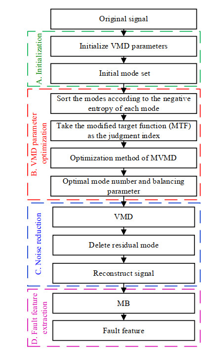
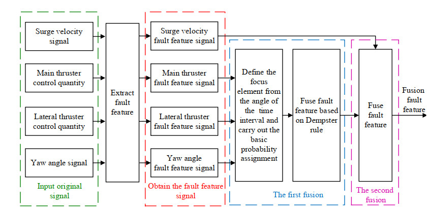
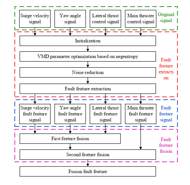
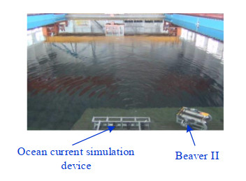
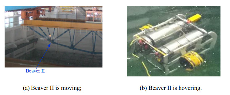
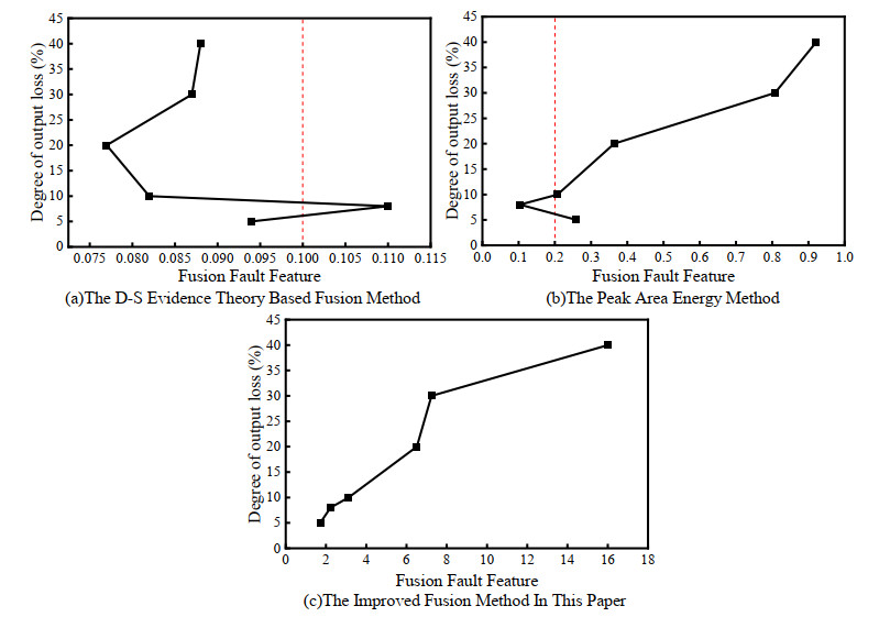
This study investigated the fault feature extraction and fusion problem for autonomous underwater vehicles with weak thruster faults. The conventional fault feature extraction and fusion method is effective when thruster faults are serious. However, for a weak thruster fault, that is, when the loss of effectiveness of thrusters is less than 10%, the following two problems occur if the conventional method is used. First, the ratio of fault features to noise features is small. Second, there is no monotonic relationship between the fusion fault features fused by the conventional method and the fault severity. In this paper, the following two methods are proposed to solve this problem: 1) Fault-feature extraction method. Based on negentropy, this method improves the evaluation index of the parameter optimization of the modified variational mode decomposition and finally enhances the fault features extracted by the modified Bayesian classification algorithm. 2) Fault-feature fusion method. To create a monotonic relationship between the fusion fault features and fault severity, this method expands the number of original signals of the traditional fusion method based on D-S evidence theory, improves the focus element of the traditional fusion method, and adopts the strategy of double fusion. Finally, the effectiveness of the proposed method was verified by pool-experiment results on Beaver II prototype.
Citation: Dacheng Yu, Mingjun Zhang, Xing Liu, Feng Yao. Fault feature extraction and fusion method for AUV with weak thruster fault based on variational mode decomposition and D-S evidence theory[J]. Mathematical Biosciences and Engineering, 2022, 19(9): 9335-9356. doi: 10.3934/mbe.2022434
This study investigated the fault feature extraction and fusion problem for autonomous underwater vehicles with weak thruster faults. The conventional fault feature extraction and fusion method is effective when thruster faults are serious. However, for a weak thruster fault, that is, when the loss of effectiveness of thrusters is less than 10%, the following two problems occur if the conventional method is used. First, the ratio of fault features to noise features is small. Second, there is no monotonic relationship between the fusion fault features fused by the conventional method and the fault severity. In this paper, the following two methods are proposed to solve this problem: 1) Fault-feature extraction method. Based on negentropy, this method improves the evaluation index of the parameter optimization of the modified variational mode decomposition and finally enhances the fault features extracted by the modified Bayesian classification algorithm. 2) Fault-feature fusion method. To create a monotonic relationship between the fusion fault features and fault severity, this method expands the number of original signals of the traditional fusion method based on D-S evidence theory, improves the focus element of the traditional fusion method, and adopts the strategy of double fusion. Finally, the effectiveness of the proposed method was verified by pool-experiment results on Beaver II prototype.

| [1] |
A. Hernandez-Sanchez, A. Poznyak, I. Chairez, O. Andrianova, Robust 3-D autonomous navigation of submersible ship using averaged sub-gradient version of integral sliding mode, Mech. Syst. Signal Proc., 149 (2021), 107169. https://10.1016/j.ymssp.2020.107169 doi: 10.1016/j.ymssp.2020.107169

|
| [2] |
K. Krasnosky, C. Roman, D. Casagrande, A bathymetric mapping and SLAM dataset with high-precision ground truth for marine robotics, Int. J. Robot. Res., 41 (2022), 12–19. https://10.1177/02783649211044749 doi: 10.1177/02783649211044749
|
| [3] |
X. Cao, H. Sun, L. Guo, Potential field hierarchical reinforcement learning approach for target search by multi-AUV in 3-D underwater environments, Int. J. Control, 93 (2020), 1677–1683. https://10.1080/00207179.2018.1526414 doi: 10.1080/00207179.2018.1526414
|
| [4] |
F. R. Wang, Z. Chen, G. B. Song, Smart crawfish: A concept of underwater multi-bolt looseness identification using entropy-enhanced active sensing and ensemble learning, Mech. Syst. Signal Proc., 149 (2021), 107186. https://10.1016/j.ymssp.2020.107186 doi: 10.1016/j.ymssp.2020.107186
|
| [5] | C. Lin, G. Han, T. Zhang, S. B. H. Shah, Y. Peng, Smart Underwater Pollution Detection Based on Graph-Based Multi-Agent Reinforcement Learning Towards AUV-Based Network ITS, IEEE Trans. Intell. Transp. Syst., (2022). https://10.1109/tits.2022.3162850 |
| [6] |
H. Wang, L. Dong, W. Song, X. Zhao, J. Xia, T. Liu, Improved U-Net-Based Novel Segmentation Algorithm for Underwater Mineral Image, Intell. Autom. Soft Comput., 32 (2022), 1573–1586. https://10.32604/iasc.2022.023994 doi: 10.32604/iasc.2022.023994
|
| [7] |
S. Gao, B. He, F. Yu, X. Zhang, T. H. Yan, C. Feng, An abnormal motion condition monitoring method based on the dynamic model and complex network for AUV, Ocean Eng., 237 (2021), 109472. https://10.1016/j.oceaneng.2021.109472 doi: 10.1016/j.oceaneng.2021.109472
|
| [8] |
F. Liu, H. Tang, J. Luo, L. Bai, H. Pu, Fault-tolerant control of active compensation toward actuator faults: An autonomous underwater vehicle example, Appl. Ocean Res., 110 (2021), 102597. https://10.1016/j.apor.2021.102597 doi: 10.1016/j.apor.2021.102597
|
| [9] |
Y. Liu, R. Bucknall, The angle guidance path planning algorithms for unmanned surface vehicle formations by using the fast marching method, Appl. Ocean Res., 59 (2016), 327–344. https://10.1016/j.apor.2016.06.013 doi: 10.1016/j.apor.2016.06.013
|
| [10] |
C. Zhu, B. Huang, B. Zhou, Y. M. Su, E. H. Zhang, Adaptive model-parameter-free fault-tolerant trajectory tracking control for autonomous underwater vehicles, ISA Trans., 114 (2021), 57–71. https://10.1016/j.isatra.2020.12.059 doi: 10.1016/j.isatra.2020.12.059
|
| [11] |
P. Wu, C. A. Harris, G. Salavasidis, A. Lorenzo-Lopez, I. Kamarudzaman, A. B. Phillips, et al., Unsupervised anomaly detection for underwater gliders using generative adversarial networks, Eng. Appl. Artif. Intell., 104 (2021), 104379. https://10.1016/j.engappai.2021.104379 doi: 10.1016/j.engappai.2021.104379
|
| [12] |
T. Lv, Z. Y. Chen, F. Yao, M. J. Zhang, Fault feature extraction method based on optimized sparse decomposition algorithm for AUV with weak thruster fault, Ocean Eng., 233 (2021), 109013. https://10.1016/j.oceaneng.2021.109013 doi: 10.1016/j.oceaneng.2021.109013
|
| [13] |
W. X. Liu, Y. J. Wang, X. Liu, M. J. Zhang, Weak thruster fault detection for AUV based on stochastic resonance and wavelet reconstruction, J. Cent. South Univ., 23 (2016), 2883–2895. https://10.1007/s11771-016-3352-1 doi: 10.1007/s11771-016-3352-1
|
| [14] |
M. Zhang, B. Yin, W. Liu, Y. Wang, Feature extraction and fusion for thruster faults of AUV with random disturbance, J. HUAZHONG UNIV. SCI. TECHNO:NAT. SCI. ED., 43 (2015), 22–26 and 54. https://10.13245/j.hust.150605 doi: 10.13245/j.hust.150605
|
| [15] | J. Q. Li, J. Li, H. Y. Chen, Y. Zhang, Y. C. Xie. Propeller feature extraction of UUVs study based on CEEMD combined with symmetric correlation. In 2020 2nd International Conference on Computer Science Communication and Network Security (CSCNS2020), (2020), 02006. https://10.1051/matecconf/202133602006 |
| [16] |
D. S. Yang, Y. H. Pang, B. W. Zhou, K. Li, Fault Diagnosis for Energy Internet Using Correlation Processing-Based Convolutional Neural Networks, IEEE Trans. Syst. Man Cybern. Syst., 49 (2019), 1739–1748. https://10.1109/tsmc.2019.2919940 doi: 10.1109/tsmc.2019.2919940
|
| [17] |
R. Wang, H. Chen, C. Guan, W. Gong, Z. Zhang, Research on the fault monitoring method of marine diesel engines based on the manifold learning and isolation forest, Appl. Ocean Res., 112 (2021), 102681. https://10.1016/j.apor.2021.102681 doi: 10.1016/j.apor.2021.102681
|
| [18] |
K. Dragomiretskiy, D. Zosso, Variational Mode Decomposition, IEEE Trans. Signal Process., 62 (2014), 531–544. https://10.1109/tsp.2013.2288675 doi: 10.1109/tsp.2013.2288675
|
| [19] | X. Jiang, J. Wang, C. Shen, J. Shi, W. Huang, Z. Zhu, et al., An adaptive and efficient variational mode decomposition and its application for bearing fault diagnosis, Struct. Health Monit., (2020), 1–18. https://10.1177/1475921720970856 |
| [20] |
J. Li, Y. Chen, Z. H. Qian, C. G. Lu, Research on VMD based adaptive denoising method applied to water supply pipeline leakage location, Measurement, 151 (2020), 107153. https://10.1016/j.measurement.2019.107153 doi: 10.1016/j.measurement.2019.107153
|
| [21] |
X. A. Yan, M. P. Jia, Application of CSA-VMD and optimal scale morphological slice bispectrum in enhancing outer race fault detection of rolling element bearings, Mech. Syst. Signal Proc., 122 (2019), 56–86. https://10.1016/j.ymssp.2018.12.022 doi: 10.1016/j.ymssp.2018.12.022
|
| [22] |
Y. J. Zhao, C. S. Li, W. L. Fu, J. Liu, T. Yu, H. Chen, A modified variational mode decomposition method based on envelope nesting and multi-criteria evaluation, J. Sound Vibr., 468 (2020), 115099. https://10.1016/j.jsv.2019.115099 doi: 10.1016/j.jsv.2019.115099
|
| [23] |
M. Zhang, B. Yin, X. Liu, J. Guo, Thruster fault identification method for autonomous underwater vehicle using peak region energy and least square grey relational grade, Adv. Mech. Eng., 7 (2015), 1–11. https://10.1177/1687814015622905 doi: 10.1177/1687814015622905
|
| [24] |
D. Zhu, B. Sun, Information fusion fault diagnosis method for unmanned underwater vehicle thrusters, IET Electr. Syst. Transp., 3 (2013), 102–111. https://10.1049/iet-est.2012.0052 doi: 10.1049/iet-est.2012.0052
|
| [25] |
X. B. Xiang, C. Y. Yu, Q. Zhang, On intelligent risk analysis and critical decision of underwater robotic vehicle, Ocean Eng., 140 (2017), 453–465. https://10.1016/j.oceaneng.2017.06.020 doi: 10.1016/j.oceaneng.2017.06.020
|
| [26] |
A. Hyvarinen, E. Oja, Independent Component Analysis: Algorithms and Applications, Neural Netw., 13 (2000), 411–430. https://https://doi.org/10.1016/S0893-6080(00)00026-5 doi: 10.1016/S0893-6080(00)00026-5
|
| [27] |
L. Han, C. W. Li, S. L. Guo, X. W. Su, Feature extraction method of bearing AE signal based on improved FAST-ICA and wavelet packet energy, Mech. Syst. Signal Proc., 62-63 (2015), 91–99. https://10.1016/j.ymssp.2015.03.009 doi: 10.1016/j.ymssp.2015.03.009
|
| [28] | G. Stefatos, A. Ben Hamza, Dynamic independent component analysis approach for fault detection and diagnosis, Expert Syst. Appl., 37 (2010), 8606–8617. https://10.1016/j.eswa.2010.06.101 |
| [29] |
L. F. Cai, X. M. Tian, A new fault detection method for non-Gaussian process based on robust independent component analysis, Process Saf. Environ. Protect., 92 (2014), 645–658. https://10.1016/j.psep.2013.11.003 doi: 10.1016/j.psep.2013.11.003
|
| [30] |
J. Yu, A nonlinear kernel Gaussian mixture model based inferential monitoring approach for fault detection and diagnosis of chemical processes, Chem. Eng. Sci., 68 (2012), 506–519. https://10.1016/j.ces.2011.10.011 doi: 10.1016/j.ces.2011.10.011
|
| [31] | Y. Deng, Deng entropy, Chaos Solitons Fractals, 91 (2016), 549–553. https://10.1016/j.chaos.2016.07.014 |
| [32] |
W. Qiao, D. Lu, A Survey on Wind Turbine Condition Monitoring and Fault Diagnosis-Part I: Components and Subsystems, IEEE Trans. Ind. Electron., 62 (2015), 6536–6545. https://10.1109/tie.2015.2422112 doi: 10.1109/tie.2015.2422112
|
| [33] | O. AlShorman, M. Irfan, N. Saad, D. Zhen, N. Haider, A. Glowacz, et al., A Review of Artificial Intelligence Methods for Condition Monitoring and Fault Diagnosis of Rolling Element Bearings for Induction Motor, Shock Vib., 2020 (2020). https://10.1155/2020/8843759 |
| [34] | O. AlShorman, F. Alkahatni, M. Masadeh, M. Irfan, A. Glowacz, F. Althobiani, et al., Sounds and acoustic emission-based early fault diagnosis of induction motor: A review study, Adv. Mech. Eng., 13 (2021). https://10.1177/1687814021996915 |
Figures(11) / Tables(4)

Dacheng Yu, Mingjun Zhang, Xing Liu, Feng Yao. Fault feature extraction and fusion method for AUV with weak thruster fault based on variational mode decomposition and D-S evidence theory[J]. Mathematical Biosciences and Engineering, 2022, 19(9): 9335-9356. doi: 10.3934/mbe.2022434


 DownLoad: