Now there is a huge variety of scenarios of prebiotic chemical evolution, culminating in the emergence of life on Earth, which demonstrates the obvious insufficiency of existing criteria for a reliable consideration of this process. This article develops the concept of thermodynamic inversion (TI concept) according to which the real succession of the formation of metabolism during the origin of life is fixed in the stages of the exit of a resting bacterial cell from anabiosis (suspended animation), just as the succession of events of phylogenesis is fixed in ontogenesis. The deepest phase of anabiosis considers by us as an intermediate state of a microorganism between non-life and life: it is no longer able to counteract the increase in entropy, but retains structural memory of the previous living state. According to the TI concept, the intermediate state between non-life and life thermodynamically corresponds to the approximate equality of the total contributions of entropy and free energy in prebiotic systems (Sc ≈ FEc). Considering such intermediate state in prebiotic systems and microorganisms as a starting point, the authors use the experimentally recorded stages of restoring the metabolic process when a resting (dormant) bacterial cell emerges from anabiosis as a guideline for identifying the sequence of metabolism origin in prebiotic systems. According to the TI concept, life originated in a pulsating updraft of hydrothermal fluid. It included four stages. 1) Self-assembly of a cluster of organic microsystems (complex liposomes). 2) Activation (formation of protocells): appearance in the microsystems a weak energy-giving process of respiration due to redox reactions; local watering in the membrane. 3) Initiation (formation of living subcells): formation of a non-enzymatic antioxidant system; dawning of the protein-synthesizing apparatus. 4) Growth (formation of living cells—progenotes): arising of the growth cell cycle; formation of the genetic apparatus.
Citation: Vladimir Kompanichenko, Galina El-Registan. Advancement of the TI concept: defining the origin-of-life stages based on the succession of a bacterial cell exit from anabiosis[J]. AIMS Geosciences, 2022, 8(3): 398-437. doi: 10.3934/geosci.2022023
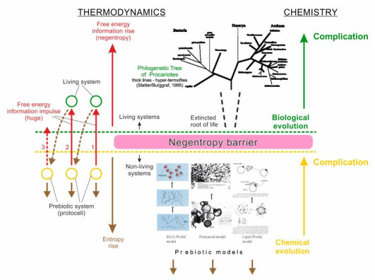
Now there is a huge variety of scenarios of prebiotic chemical evolution, culminating in the emergence of life on Earth, which demonstrates the obvious insufficiency of existing criteria for a reliable consideration of this process. This article develops the concept of thermodynamic inversion (TI concept) according to which the real succession of the formation of metabolism during the origin of life is fixed in the stages of the exit of a resting bacterial cell from anabiosis (suspended animation), just as the succession of events of phylogenesis is fixed in ontogenesis. The deepest phase of anabiosis considers by us as an intermediate state of a microorganism between non-life and life: it is no longer able to counteract the increase in entropy, but retains structural memory of the previous living state. According to the TI concept, the intermediate state between non-life and life thermodynamically corresponds to the approximate equality of the total contributions of entropy and free energy in prebiotic systems (Sc ≈ FEc). Considering such intermediate state in prebiotic systems and microorganisms as a starting point, the authors use the experimentally recorded stages of restoring the metabolic process when a resting (dormant) bacterial cell emerges from anabiosis as a guideline for identifying the sequence of metabolism origin in prebiotic systems. According to the TI concept, life originated in a pulsating updraft of hydrothermal fluid. It included four stages. 1) Self-assembly of a cluster of organic microsystems (complex liposomes). 2) Activation (formation of protocells): appearance in the microsystems a weak energy-giving process of respiration due to redox reactions; local watering in the membrane. 3) Initiation (formation of living subcells): formation of a non-enzymatic antioxidant system; dawning of the protein-synthesizing apparatus. 4) Growth (formation of living cells—progenotes): arising of the growth cell cycle; formation of the genetic apparatus.

| [1] | Oparin AI (1957) Origin of Life on the Earth. Moscow: Nauka. |
| [2] | Fox SW, Bahn PR, Pappelis A, et al. (1996) Experimental retracement of terrestrial origin of an excitable cell: Was it predictable? Chemical Evolution: Physics of the Origin and Evolution of Life, Basingstoke, UK: Springer Nature, 21-32. https://doi.org/10.1007/978-94-009-1712-5_2 |
| [3] |
Ikehara K (2015)[GADV]-Protein World Hypothesis on the Origin of Life. Orig Life Evol Biosph 44: 299-302. https://doi.org/10.1007/s11084-014-9383-4 doi: 10.1007/s11084-014-9383-4

|
| [4] | Joice GF, Orgel LE (1993) Prospects for understanding the origin of the RNA world. The RNA World, New York: Gold Spring Harbor laboratory Press, 1-25. |
| [5] | Deamer DW (2004) Prebiotic amphiphilic compounds, In: Seckbach J, Origins. Cellular Origin, Life in Extreme Habitats and Astrobiology, Dordrecht, The Netherlands: Springer, 75-89. https://doi.org/10.1007/1-4020-2522-X_6 |
| [6] |
Luisi PL (2000) The relevance of supramolecular chemistry for the origin of life. Adv Supramol Chem 6: 287-307. https://doi.org/10.1016/S1068-7459(00)80009-0 doi: 10.1016/S1068-7459(00)80009-0
|
| [7] |
Ehrenfreund P, Rasmussen S, Cleaves J, et al. (2006) Experimentally tracing the key steps in the origin of life: The aromatic world. Astrobiology 6: 490-520. https://doi.org/10.1089/ast.2006.6.490 doi: 10.1089/ast.2006.6.490
|
| [8] |
Huber C, Wächtershäuser G (1998) Peptides by activation of amino acids with CO on (Ni, Fe)S surfaces: implications for the origin of life. Science 281: 670-672. https://doi.org/10.1126/science.281.5377.670 doi: 10.1126/science.281.5377.670
|
| [9] |
Kurihara K, Tamura M, Shohda Ki, et al. (2011) Self-reproduction of supramolecular giant vesicles combined with the amplification of encapsulated DNA. Nature Chem 3: 775-781. https://doi.org/10.1038/nchem.1127 doi: 10.1038/nchem.1127
|
| [10] | Sugawara T, Kurihara K, Suzuki K (2012) Constructive approach toward protocells. In: Mikhailov A, Engineering of chemical complexity, 1-17. https://doi.org/10.1142/9789814390460_0018 |
| [11] | Deamer DW (2011) First Life. Berkeley CA: University of California Press. |
| [12] |
Damer B, Deamer D (2020) The Hot Spring Hypothesis for an Origin of Life. Astrobiology 20: 429-452. https://doi.org/10.1089/ast.2019.2045 doi: 10.1089/ast.2019.2045
|
| [13] |
Holm NG, Andersson E (2005) Hydrothermal simulation experiments as a tool for studies for the origin of life on Earth and other terrestrial planets: a review. Astrobiology 5: 444-460. https://doi.org/10.1089/ast.2005.5.444 doi: 10.1089/ast.2005.5.444
|
| [14] |
Saladino R, Crestini C, Pino S, et al. (2012) Formamide and the origin of life. Phys Life Rev 9: 84-104. https://doi.org/10.1016/j.plrev.2011.12.002 doi: 10.1016/j.plrev.2011.12.002
|
| [15] |
Gaylor M, Miro P, Vlaisavljevich B, et al. (2021) Plausible Emergence and Self Assembly of a Primitive Phospholipid from Reduced Phosphorus on the Primordial Earth. Orig Life Evol Biosph 51: 185-213. https://doi.org/10.1007/s11084-021-09613-4 doi: 10.1007/s11084-021-09613-4
|
| [16] |
Miller SL (1953) Production of Amino Acids Under Possible Primitive Earth Conditions. Science 117: 528-529. https://doi.org/10.1126/science.117.3046.528 doi: 10.1126/science.117.3046.528
|
| [17] |
Markhinin EK, Podkletnov NE (1977) The phenomenon of formation of prebiological compounds in volcanic processes. Orig Life Evol Biosph 8: 225-235. https://doi.org/10.1007/BF00930684 doi: 10.1007/BF00930684
|
| [18] |
Yokoyama S, Koyama A, Nemoto A, et al. (2003) Amplification of diverse catalytic properties of evolving molecules in a simulated hydrothermal environment. Orig Life Evol Biosph 33: 589-595. https://doi.org/10.1023/a:1025741430748 doi: 10.1023/A:1025741430748
|
| [19] |
Kawamura K, Shimahashi M (2008) One-step formation of oligopeptide-like molecules from Glu and Asp in hydrothermal environments. Naturwissenschaften 95: 449-454. https://doi.org/10.1007/s00114-008-0342-7 doi: 10.1007/s00114-008-0342-7
|
| [20] |
Cleaves HJ, Aubrey AD, Bada JL (2009) An evaluation of critical parameters for abiotic peptide synthesis in submarine hydrothermal systems. Orig Life Evol Biosph 39: 109-126. https://doi.org/10.1007/s11084-008-9154-1 doi: 10.1007/s11084-008-9154-1
|
| [21] |
Deamer DW (1985) Boundary structures are formed by organic components of the Murchison carbonaceous chondrite. Nature 317: 792-794. https://doi.org/10.1038/317792a0 doi: 10.1038/317792a0
|
| [22] |
Martins Z, Botta O, Fogel ML, et al. (2008) Extraterrestrial nucleobases in the Murchison meteorite. Earth Plan Sci Let 270: 130-136. https://doi.org/10.1016/j.epsl.2008.03.026 doi: 10.1016/j.epsl.2008.03.026
|
| [23] |
Joyce G (2002) The antiquity of RNA-world evolution. Nature 418: 214-221. https://doi.org/10.1038/418214a doi: 10.1038/418214a
|
| [24] |
Woese CR (1987) Microbial evolution. Microbiol Rev 51: 221-270. doi: 10.1128/mr.51.2.221-271.1987
|
| [25] | Kompanichenko VN (2002) Life as High-Organized Form of Intensified Resistance to Destructive Processes, Fundamentals of Life, Paris: Elsevier, 111-124. |
| [26] |
Kompanichenko VN (2008) Three stages of the origin-of-life process: bifurcation, stabilization and inversion. Int J Astrobiology 7: 27-46. https://doi.org/10.1017/S1473550407003953 doi: 10.1017/S1473550407003953
|
| [27] |
Kompanichenko VN (2012) Inversion concept of the origin of life. Orig Life Evol Biosph 42: 153-178. https://doi.org/10.1007/s11084-012-9279-0 doi: 10.1007/s11084-012-9279-0
|
| [28] | Kompanichenko VN (2017) Thermodynamic Inversion: Origin of Living Systems, Cham (Switzerland): Springer International Publishing. https://doi.org/10.1007/978-3-319-53512-8 |
| [29] |
Kompanichenko V (2019) The Rise of A Habitable Planet: Four Required Conditions for the Origin of Life in the Universe. Geosciences 9: 92. https://doi.org/10.3390/geosciences9020092 doi: 10.3390/geosciences9020092
|
| [30] |
Kompanichenko V (2020) Thermodynamic Jump from Prebiotic Microsystems to Primary Living Cells. Sci 2: 14. https://doi.org/10.3390/sci2010014 doi: 10.3390/sci2010014
|
| [31] | Feistel R, Ebeling W (2011) Physics of Self-organization and Evolution, VCH: Wiley. |
| [32] | Bukharin OV, Gintsburg AP, Romanova YM, et al. (2005) Survival mechanisms of bacteria, Moscow: Medicine. |
| [33] |
El-Registan GI, Mulyukin AL, Nikolaev YA, et al. (2006) Adaptogenic functions of extracellular autoregulators of mmicroorganisms. Mikrobiologiya 75: 380-389. https://doi.org/10.1134/S0026261706040035 doi: 10.1134/S0026261706040035
|
| [34] | Prigogine I, Nicolis G (1977) Self-organization in Nonequilibrium Systems, New York: Wiley. |
| [35] | Prigogine I, Stengers I (1984) Order out of chaos, New York: Bantam. |
| [36] |
Prigogine I (1989) The philosophy of instability. Futures 21: 396-400. https://doi.org/10.1016/S0016-3287(89)80009-6 doi: 10.1016/S0016-3287(89)80009-6
|
| [37] | Haken H (1978) Synergetics. Berlin, New York: Springer-Verlag. |
| [38] | Ebeling W, Engel A, Feistel R (1990) Physik der Evolutionsprozesse, Berlin: Akademie-Verlag. |
| [39] | Kompanichenko VN (2004) Systemic approach to the origin of life. Front Perspect 13: 22-40. https://www.researchgate.net/publication/292712728 |
| [40] | Selye H (1974) Stress without distress, Philadelfia & New York: JB Lippincott Company. |
| [41] |
Herkovits J (2006) Evoecotoxicology: Environmental Changes and Life Features Development during the Evolutionary Process—the Record of the Past at Developmental Stages of Living Organisms. Environ Health Perspect 114. https://doi.org/10.1289/ehp.8633 doi: 10.1289/ehp.8633
|
| [42] | Corliss JB, Baross JA, Hoffman SE (1981) An hypothesis concerning the relationship between submarine hot springs and the origin of life on the Earth. Oceanol Acta 4: 59-69. |
| [43] |
Marshall WL (1994) Hydrothermal synthesis of amino acids. Geochim Cosmochim Acta 58: 2099-2106. https://doi.org/10.1016/0016-7037(94)90288-7 doi: 10.1016/0016-7037(94)90288-7
|
| [44] |
Washington J (2000) The possible role of volcanic aquifers in prebiotic genesis of organic compounds and RNA. Orig Life Evol Biosph 30: 53-79. https://doi.org/10.1023/A:1006692606492 doi: 10.1023/A:1006692606492
|
| [45] |
Martin W, Russell JM (2007) On the origin of biochemistry at an alkaline hydrothermal vent. Philos Trans R Soc B 362: 1887-1925. https://doi.org/10.1098/rstb.2006.1881 doi: 10.1098/rstb.2006.1881
|
| [46] | Kolb VM (2016) Green Organic Chemistry and Its Interdisciplinary Applications, Boca Raton, CRC Press. https://doi.org/10.1201/9781315371856 |
| [47] |
Van Kranendonk MJ, Baumgartner R, Djokic T, et al. (2021) Elements for the Origin of Life on Land: A Deep-Time Perspective from the Pilbara Craton of Western Australia. Astrobiology 21: 39-59. https://doi.org/10.1089/ast.2019.2107 doi: 10.1089/ast.2019.2107
|
| [48] |
Deamer D (2021) Where Did Life Begin? Testing Ideas in Prebiotic Analogue Conditions. Life 11: 134. https://doi.org/10.3390/life11020134 doi: 10.3390/life11020134
|
| [49] |
Russell MJ (2021) The "Water Problem"(sic), the Illusory Pond and Life's Submarine Emergence—A Review. Life 11: 429. https://doi.org/10.3390/life11050429 doi: 10.3390/life11050429
|
| [50] | Kralj P (2001) Das Thermalwasser-System des Mur-Beckens in Nordost-Slowenien. Mitteilungen zur Ingenieurgeologie und Hydrogeologie, 81: 82, RWTH Aachen, Germany. |
| [51] |
Kralj P, Kralj P (2000) Thermal and mineral waters in north-eastern Slovenia. Environ Geol 39: 488-500. https://doi.org/10.1007/s002540050455 doi: 10.1007/s002540050455
|
| [52] | Kiryukhin AV, Lesnyikh MD, Polyakov AY. (2002) Natural hydrodynamic mode of the Mutnovsky geothermal reservoir and its connection with seismic activity. Volc Seis 1: 51-60. |
| [53] |
Kompanichenko VN, Poturay VA, Shlufman KV (2015) Hydrothermal systems of Kamchatka are models of the prebiotic environment. Orig Life Evol Biosph 45: 93-103. https://doi.org/10.1007/s11084-015-9429-2 doi: 10.1007/s11084-015-9429-2
|
| [54] |
Ross David S, Deamer D (2016) Dry/Wet Cycling and the Thermodynamics and Kinetics of Prebiotic Polymer Synthesis. Life 6: 28. https://doi.org/10.3390/life6030028 doi: 10.3390/life6030028
|
| [55] |
Deamer D, Damer B, Kompanichenko V (2019) Hydrothermal Chemistry and the Origin of Cellular Life. Astrobiology 19: 1523-1537. https://doi.org/10.1089/ast.2018.1979 doi: 10.1089/ast.2018.1979
|
| [56] | Huxley IS (1942) Evolution: the modern synthesis, London: George Allen and Unwin. |
| [57] | McCollom TM, Seewald JS (2001) A reassessment of the potential for reduction of dissolved CO2 to hydrocarbons during serpentinization of olivine. Geochim Cosmochim Acta 65: 3769-3778. Available from: https://www.elibrary.ru/item.asp?id=826854 |
| [58] | Shock EL, McCollom TM, Schulte MD (1998) The emergence of metabolism from within hydrothermal systems, Thermophiles: The Keys to Molecular Evolution and the Origin of Life, Washington: Taylor and Francis, 59-76. |
| [59] |
Rushdi AI, Simoneit BRT (2004) Condensation reactions and formation of amides, esters, and nitriles under hydrothermal conditions. Astrobiology 4: 211-224. https://doi.org/10.1089/153110704323175151 doi: 10.1089/153110704323175151
|
| [60] | Simoneit BRT (2003) Petroleum generation, extraction and migration and abiogenic synthesis in hydrothermal systems, Natural and Laboratory Simulated Thermal Geochemical Processes, Netherlands: Kluwer, 1-30. https://doi.org/10.1007/978-94-017-0111-2_1 |
| [61] |
Simoneit BRT (2004) Prebiotic organic synthesis under hydrothermal conditions: an overview. Adv Space Res 33: 88-94. https://doi.org/10.1016/j.asr.2003.05.006 doi: 10.1016/j.asr.2003.05.006
|
| [62] | Fox S, Dose K (1975) Molecular Evolution and the Origin of Life, New York: Dekker. |
| [63] |
Larralde R, Robertson M, Miller S (1995) Rates of decomposition of ribose and other sugars: implications for chemical evolution. Proc Natl Acad Sci USA 92: 8158-8160. https://doi.org/10.1073/pnas.92.18.8158 doi: 10.1073/pnas.92.18.8158
|
| [64] |
Vergne J, Dumas L, Decout JL, et al. (2000) Possible prebiotic catalysts formed from adenine and aldehyde. Planet Space Sci 48: 1139-1142. https://doi.org/10.1016/S0032-0633(00)00087-8 doi: 10.1016/S0032-0633(00)00087-8
|
| [65] |
Kazem K, Lovley DR (2003) Extending the Upper Temperature Limit for Life. Science 301: 934. https://doi.org/10.1126/science.1086823 doi: 10.1126/science.1086823
|
| [66] |
Varfolomeev SD (2007) Kinetic models of prebiological evolution of macromoleculer. Thermocycle as the motive force of the process. Mendeleev Commun 17: 7-9. https://doi.org/10.1016/j.mencom.2007.01.003 doi: 10.1016/j.mencom.2007.01.003
|
| [67] |
Osipovich DC, Barratt C, Schwartz PM (2009) Systems chemistry and Parrondo's paradox: computational models of thermal cycling. New J Chem 33: 1981-2184. https://doi.org/10.1039/b900288j doi: 10.1039/b919103h
|
| [68] |
Singh SV, Vishakantaiah J, Meka JK, et al. (2020) Shock Processing of Amino Acids Leading to Complex Structures—Implications to the Origin of Life. Molecules 25: 5634. https://doi.org/10.3390/molecules25235634 doi: 10.3390/molecules25235634
|
| [69] |
Surendra VS, Jayaram V, Muruganantham M, et al. (2021) Complex structures synthesized in shock processing of nucleobases—implications to the origins of life. Int J Astrobiology 20: 285-293. https://doi.org/10.1017/S1473550421000136 doi: 10.1017/S1473550421000136
|
| [70] | Mazur P (2004) Principles of cryobiology, Life in the frozen state, Boca Raton: CRC Press, 3-65. https://doi.org/10.1201/9780203647073 |
| [71] |
Clarke A, Morris GJ, Fonesca F, et al. (2013) A low temperature limit for life on Earth. PLoS One 8: e66207. https://doi.org/10.1371/journal.pone.0066207 doi: 10.1371/journal.pone.0066207
|
| [72] |
Fonesca F, Meneghel J, Cenard S, et al. (2016) Determination of Intracellular Vitrification Temperatures for Unicellular Microorganisms under Condition Relevant for Cryopreservation. PLoS One 11: e0152939. https://doi.org/10.1371/journal.pone.0152939 doi: 10.1371/journal.pone.0152939
|
| [73] | Schrodinger E (1944) What is life? Cambridge University Press. |
| [74] |
Frenkel-Krispin D, Minsky A (2006) Nucleoid organization and the maintenance of DNA integrity in E. coli, B. subtiles and D. radiodurans. J Struct Biol 156: 311-319. https://doi.org/10.1016/j.jsb.2006.05.014 doi: 10.1016/j.jsb.2006.05.014
|
| [75] |
Dadinova LA, Chsnokov IM, Kamyshinsky RA, et al. (2019) Protective Dps-DNA co-crystallization in stressed cells: an in vitro structural study by small-angle X-ray scattering and cryoelectron tomography. FEBS Letters 593: 1360-1371. https://doi.org/10.1002/1873-3468.13439 doi: 10.1002/1873-3468.13439
|
| [76] |
Loiko NG, Suzina NE, Soina VS, et al. (2017) Biocrysteline Structure in the Nucleoids of the Stationary and Dormant Prokaryotic Cells. Microbiology 86: 714-727. https://doi.org/10.1134/S002626171706011X doi: 10.1134/S002626171706011X
|
| [77] |
Parry BR, Surovtsev Ⅳ, Cabeen MT, et al. (2014) The Bacterial clytoplasm Has Glass-like Properties and Fluidized by Metabolic Activity. Cell 156: 183-194. https://doi.org/10.1016/j.cell.2013.11.028 doi: 10.1016/j.cell.2013.11.028
|
| [78] |
Mourão MA, Hakim JB, Schnell S (2014) Connecting the Dots: The Effects of Macromolecular Crowding on Cell Physiology. Biophys J 107: 2761-2766. https://doi.org/10.1016/j.bpj.2014.10.051 doi: 10.1016/j.bpj.2014.10.051
|
| [79] |
Mika JT, van der Bogaart G, Veenhoff L, et al. (2010) Molecular sieving properties of the cytoplasm of Escherichia coli and consequences of osmotic stress: Molecule diffusion and barriers in the cytoplasm. Mol Microbiol 77: 200-207. https://doi.org/10.1111/j.1365-2958.2010.07201.x doi: 10.1111/j.1365-2958.2010.07201.x
|
| [80] |
Antipov S, Turishchev S, Purtov Y, et al. (2017) The oligomeric forms of the Escherichia coli Dps protein depends on the availability of Iron Ions. Molecules 22: 1904. https://doi.org/10.3390/molecules22111904 doi: 10.3390/molecules22111904
|
| [81] | Shapiro JA, Dworkin M (1997) Bacteria as multicellular organisms, Oxford University Press. |
| [82] |
Lewis K (2010) Persister cells. Annu Rev Microbiol 64: 357-372. https://doi.org/10.1146/annurev.micro.112408.134306 doi: 10.1146/annurev.micro.112408.134306
|
| [83] |
Podlesek Z, Butala M, Šakanovié A, et al. (2016) Antibiotic induced bacterial lysis provided a reservoir of persisters. Antonie van Leeuwenhoek 109: 523-528. https://doi.org/10.1007/s10482-016-0657-x doi: 10.1007/s10482-016-0657-x
|
| [84] |
Selye HA (1936) A syndrome produced by diverse nocuous agents. Nature 138: 32. https://doi.org/10.1038/138032a0 doi: 10.1038/138032a0
|
| [85] | Tkachenko AG (2012) Molecular mechanisms of stress responses in microorganisms. Ekaterinburg: IEGM UB RAS (In Russian). |
| [86] |
Fukua WC, Winans SC, Greenberg EP (1994) Quorum sensing in bacteria: the LuxJ family of cell density—responsive transcription regulators. J Bacteriol 176: 269-275. https://doi.org/10.1128/jb.176.2.269-275.1994 doi: 10.1128/jb.176.2.269-275.1994
|
| [87] |
Imlay JA (2003) Pathways of oxidative damage. Annu Rev Microbiol 57: 395-418. https://doi.org/10.1146/annurev.micro.57.030502.090938 doi: 10.1146/annurev.micro.57.030502.090938
|
| [88] |
Imlay JA (2008) Cellular Defenses against Superoxide and Hydrogen Peroxide. Annu Rev Biochem 77: 755-776. https://doi.org/10.1146/annurev.biochem.77.061606.161055 doi: 10.1146/annurev.biochem.77.061606.161055
|
| [89] |
Loiko NG, Kozlova AN, Nikolaev YA, et al. (2015) Effect of stress on emergence of antibiotic-tolerant Escherichia coli cells. Mikrobiologiya 84: 595-609. https://doi.org/10.1134/S0026261715050148 doi: 10.1134/S0026261715050148
|
| [90] |
Mayer MP, Bukau B (2005) Hsp 70 chaperones: cellular function and molecular mechnisms. Cell Mol Life Sci 62: 670-684. https://doi.org/10.1007/s00018-004-4464-6 doi: 10.1007/s00018-004-4464-6
|
| [91] |
Krupyansky YF, Abdulnasyrov EG, Loiko NG, et al. (2012) Possible mechanisms of influence of hexylresorcinol on the structural-dynamic and functional properties of the lysozyme protein. Russ J Phys Chem B 6: 301-314. https://doi.org/10.1134/S1990793112020078 doi: 10.1134/S1990793112020078
|
| [92] | Martirosova EI, Karpekina TA, El-Registan GI (2004) Modification of enzymes by natural chemical chaperones of microorganisms. Mikrobiologiya 73: 708-715. |
| [93] | Stepanenko IY, Strakhovskaya MG, Belenikina NS, et al. (2004) Protection of Saccharomyces cerevisiae with alkyloxybenzenes from oxidative and radiation damage. Mikrobiologiya 73: 204-210. |
| [94] |
Azam TA, Hiraga S, Jshihama A (2000) Two types of localization of the DNA-binding protein within the Escherichia coli nucleoid. Genes Cells 5: 613-626. https://doi.org/10.1046/j.1365-2443.2000.00350.x doi: 10.1046/j.1365-2443.2000.00350.x
|
| [95] |
Frenkel-Krispin D, Levin-Zaidman S, Shimoni E, et al. (2001) Regulated phase Transitions of bacterial chromatin: a non-enzymatic pathway for generic DNA protection. EMBO J 20: 1184-1191. https://doi.org/10.1093/emboj/20.5.1184 doi: 10.1093/emboj/20.5.1184
|
| [96] |
Karas VA, Westerlaken I, Meyer AS (2013) Application of an in vitro DNA protection assay to visualize stress mediation properties of the Dps protein. J Vis Exp 75: E50390. https://doi.org/10.3791/50390 doi: 10.3791/50390
|
| [97] |
Grant SS, Hung DT (2013) Persistent bacterial infections, antibiotic tolerance, and oxidative stress response. Virulence 4: 273-283. https://doi.org/10.4161/viru.23987 doi: 10.4161/viru.23987
|
| [98] |
Mysyakina IS, Sergeeva YE, Sorokin VV, et al. (2014) Lipid and elemental composition of indicators of the physiological state of Sporangiospores in Mucor hiemalis cultures of different ages. Microbiology 83: 110-118. https://doi.org/10.1134/S0026261714020155 doi: 10.1134/S0026261714020155
|
| [99] |
Ignatow DK, Salina EG, Fursov MV, et al. (2015) Dormant non-culturable Mycobacterium tuberculosis retains stable low-abundant mRNA. BMC Genomics 16: 954. https://doi.org/10.1186/s12864-015-2197-6 doi: 10.1186/s12864-015-2197-6
|
| [100] |
Sanchez-Avila JI, Garcia Sanchez BE, Vara-Castro BM, et al. (2021) Disrtibution and origin of organic compounds in the condensates from a Mexican high-temperature hydrothermal field. Geothermics 89: 101980. https://doi.org/10.1016/j.geothermics.2020.101980 doi: 10.1016/j.geothermics.2020.101980
|
| [101] | Mukhin LM, Bondarev VB, Vakin EA, et al. (1979) Amino acids in hydrothermal systems in Southern Kamchatka. Doklady Acad Sci USSR 244: 974-977. |
| [102] | Kompanichenko VN, Avchenko OV (2015) Thermodynamic calculations of the parameters of hydrothermal environment in the modelling of biosphere origin. Reg Probl 18: 5-13. Available from: https://readera.org/14328903 |
| [103] |
Barge LM, Branscomb E, Brucato JR, et al. (2017) Thermodynamics, Disequilibrium, Evolution: Far-From-Equilibrium Geological and Chemical Considerations for Origin-Of-Life Research. Orig Life Evol Biosph 47: 39-56. https://doi.org/10.1007/s11084-016-9508-z doi: 10.1007/s11084-016-9508-z
|
| [104] |
Hengeveld R, Fedonkin MA (2007) Bootstrapping the energy flow in the beginning of life. Acta Biotheor 55: 181-226. https://doi.org/10.1007/s10441-007-9019-4 doi: 10.1007/s10441-007-9019-4
|
| [105] | Fedonkin MA (2008) Ancient biosphere: The origin, trends and events. Russ Jour Earth Sci 10: 1-9. Available from: https://www.elibrary.ru/item.asp?id=21653921. |
| [106] |
Galimov EM (2006) Phenomenon of Life: between equilibrium and non-linearity. Orig Life Evol Biosph 34: 599-613. https://doi.org/10.1023/b:orig.0000043131.86328.9d doi: 10.1023/b:orig.0000043131.86328.9d
|
| [107] |
Kompanichenko VN (2014) Emergence of biological organization through thermodynamic inversion. Front Biosci E 6: 208-224. https://doi.org/10.2741/e703 doi: 10.2741/e703
|
| [108] |
Cruz-Rosas HI, Riquelme F, Ramírez-Padrón A, et al. (2020) Molecular shape as a key source of prebiotic information. J Theor Biol 499: 110316. https://doi.org/10.1016/j.jtbi.2020.110316 doi: 10.1016/j.jtbi.2020.110316
|
| [109] | Abel DL (2015) Primordial Prescription: the most plaguing problem of life origin science, New York: LongView Press-Academic. |
| [110] |
Knauth LP, Lowe DR (2003) High Archean climatic temperature inferred from oxygen isotope geochemistry of cherts in the 3.5 Ga Swaziland Supergroup, South Africa. GSA Bull 115: 566-580. https://doi.org/10.1130/0016-7606(2003)115 < 0566:HACTIF > 2.0.CO; 2 doi: 10.1130/0016-7606(2003)115 < 0566:HACTIF > 2.0.CO; 2
|


Figures(4)

Vladimir Kompanichenko, Galina El-Registan. Advancement of the TI concept: defining the origin-of-life stages based on the succession of a bacterial cell exit from anabiosis[J]. AIMS Geosciences, 2022, 8(3): 398-437. doi: 10.3934/geosci.2022023


 DownLoad: