Safety action over oscillations of a beam excited by moving load via a new active vibration controller

Hany Bauomy; Hany Bauomy

doi:10.3934/mbe.2023238

Mathematical Biosciences and Engineering

2023, Volume 20, Issue 3: 5135-5158. doi: 10.3934/mbe.2023238

Previous Article Next Article

Research article Special Issues

Safety action over oscillations of a beam excited by moving load via a new active vibration controller

Hany Bauomy ^{1,2
,
,}

1.
Department of Mathematics, College of Arts and Science in Wadi Addawasir, Prince Sattam Bin Abdulaziz University, P.O. Box 54, Wadi Addawasir 11991, Saudi Arabia
2.
Department of Mathematics, Faculty of Science, Zagazig University, Zagazig 44519, Egypt

Academic Editor: Jesús Martín Vaquero

Received: 15 October 2022 Revised: 04 December 2022 Accepted: 18 December 2022 Published: 09 January 2023

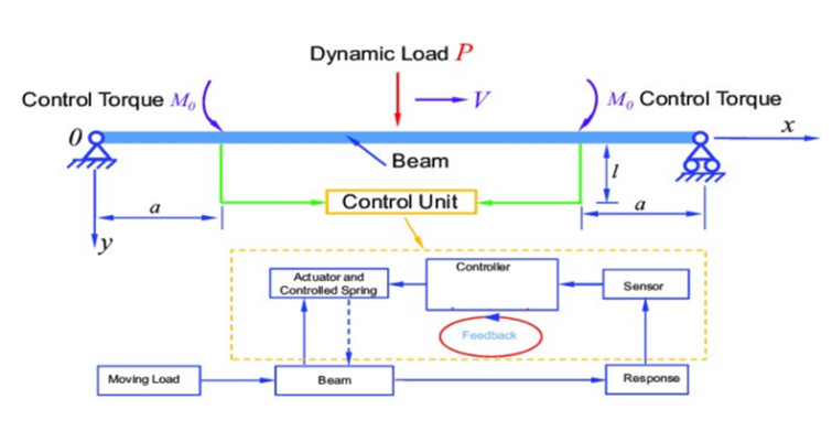
This paper presents a mixed active controller (NNPDCVF) that combines cubic velocity feedback with a negative nonlinear proportional derivative to reduce the nonlinear vibrating behavior of a nonlinear dynamic beam system. Multiple time-scales method treatment is produced to get the mathematical solution of the equations for the dynamical modeling with NNPDCVF controller. This research focuses on two resonance cases which are the primary and 1/2 subharmonic resonances. Time histories of the primary system and the controller are shown to demonstrate the reaction with and without control. The time-history response, as well as the impacts of the parameters on the system and controller, are simulated numerically using the MATLAB program. Routh-Hurwitz criterion is used to examine the stability of the system under primary resonance. A numerical simulation, using the MATLAB program software, is obtained to show the time-history response, the effect of the parameters on the system and the controller. An investigation is done into how different significant effective coefficients affect the resonance's steady-state response. The results demonstrate that the main resonance response is occasionally impacted by the new active feedback control's ability to effectively attenuate amplitude. Choosing an appropriate control Gaining quantity can enhance the effectiveness of vibration control by avoiding the primary resonance zone and unstable multi-solutions. Optimum control parameter values are calculated. Validation curves are provided to show how closely the perturbation and numerical solutions are related.
- perturbation technique,
- beam,
- stability,
- resonance case,
- mixed controllers
Citation: Hany Bauomy. Safety action over oscillations of a beam excited by moving load via a new active vibration controller[J]. Mathematical Biosciences and Engineering, 2023, 20(3): 5135-5158. doi: 10.3934/mbe.2023238

Related Papers:

Abstract

This paper presents a mixed active controller (NNPDCVF) that combines cubic velocity feedback with a negative nonlinear proportional derivative to reduce the nonlinear vibrating behavior of a nonlinear dynamic beam system. Multiple time-scales method treatment is produced to get the mathematical solution of the equations for the dynamical modeling with NNPDCVF controller. This research focuses on two resonance cases which are the primary and 1/2 subharmonic resonances. Time histories of the primary system and the controller are shown to demonstrate the reaction with and without control. The time-history response, as well as the impacts of the parameters on the system and controller, are simulated numerically using the MATLAB program. Routh-Hurwitz criterion is used to examine the stability of the system under primary resonance. A numerical simulation, using the MATLAB program software, is obtained to show the time-history response, the effect of the parameters on the system and the controller. An investigation is done into how different significant effective coefficients affect the resonance's steady-state response. The results demonstrate that the main resonance response is occasionally impacted by the new active feedback control's ability to effectively attenuate amplitude. Choosing an appropriate control Gaining quantity can enhance the effectiveness of vibration control by avoiding the primary resonance zone and unstable multi-solutions. Optimum control parameter values are calculated. Validation curves are provided to show how closely the perturbation and numerical solutions are related.

References

[1]	P. Avitable, Twenty years of structural dynamic modification-a review, Sound Vib., 37 (2003), 14–27.
[2]	M. Nad, Modification of modal characteristics of vibrating structural elements, Scientific Monographs, Köthen, 2010.
[3]	M. Sága, M. Žmindák, V. Deký;š, A. Sapietová, Š. Segľa, Selected methods for the analysis and synthesis of mechanical systems, VTS ZU, Zilina, (2009).
[4]	D. Stăncioiu, H. Ouyang, J. E. Mottershead, Vibration of a beam excited by a moving oscillator considering separation and reattachment, J. Sound Vib., 310 (2008), 1128–1140. https://doi.org/10.1016/j.jsv.2007.08.019 doi: 10.1016/j.jsv.2007.08.019
[5]	L. Sun, Dynamic displacement response of beam-type structures to moving line loads, Int. J. Solids Struct., 38 (2001), 8869–8878. https://doi.org/10.1016/s0020-7683(01)00044-0 doi: 10.1016/s0020-7683(01)00044-0
[6]	S. Y. Lee, S. S. Yhim, Dynamic analysis of composite plates subjected to multi-moving loads based on a third order theory, Int. J. Solids Struct., 41 (2004), 4457–4472. https://doi.org/10.1016/j.ijsolstr.2004.03.021 doi: 10.1016/j.ijsolstr.2004.03.021
[7]	A.V. Pesterev, L. A. Bergman, A contribution to the moving mass problem, J. Vib. Acoust., 120 (1998), 824–826. https://doi.org/10.1115/1.2893904 doi: 10.1115/1.2893904
[8]	N. Azizi, M. M. Saadatpour, M. Mahzoon, Using spectral element method for analyzing continuous beams and bridges subjected to a moving load, Appl. Math. Model., 36 (2012), 3580–3592. https://doi.org/10.1016/j.apm.2011.10.019 doi: 10.1016/j.apm.2011.10.019
[9]	M. Dehestani, M. Mofid, A. Vafai, Investigation of critical influential speed for moving mass problems on beams, Appl. Math. Model., 33 (2009), 3885–3895. https://doi.org/10.1016/j.apm.2009.01.003 doi: 10.1016/j.apm.2009.01.003
[10]	A. Nikkhoo, F. R. Rofooei, M. R. Shadnam, Dynamic behavior and modal control of beams under moving mass, J. Sound Vib., 306 (2007), 712–724. https://doi.org/10.1016/j.jsv.2007.06.008 doi: 10.1016/j.jsv.2007.06.008
[11]	S. Marchesiello, A. Fasana, L. Garibaldi, B. A. D. Piombo, Dynamics of multi-span continuous straight bridges subject to multi-degrees of freedom moving vehicle excitation, J. Sound Vib., 224 (1999), 541–561. https://doi.org/10.1006/jsvi.1999.2197 doi: 10.1006/jsvi.1999.2197
[12]	L. Fryba, Vibration of Solids and Structures Under Moving Loads, Thomas Telford, 1999. https://doi.org/10.1680/vosasuml.35393.0027
[13]	Z. C. Qiu, X. M. Zhang, H. X. Wu, H. H. Zhang, Optimal placement and active vibration control for piezoelectric smart flexible cantilever plate, J. Sound Vib., 301 (2007), 521–543. https://doi.org/10.1016/j.jsv.2006.10.018 doi: 10.1016/j.jsv.2006.10.018
[14]	J. J. Liao, A. P. Wang, C. M. Ho, Y. D. Hwang, A robust control of a dynamic beam structure with time delay effect, J. Sound Vib., 252 (2002), 835–847. https://doi.org/10.1006/jsvi.2001.3772 doi: 10.1006/jsvi.2001.3772
[15]	C. M. Casado, I. M. Díaz, J. Sebastián, A. V. Poncela, A. Lorenzana, Implementation of passive and active vibration control on an in-service footbridge, Struct. Control Health Monit., 20 (2013), 70–87. https://doi.org/10.1002/stc.471 doi: 10.1002/stc.471
[16]	D. Younesian, E. Esmailzadeh, R. Sedaghati, Passive vibration control of beams subjected to random excitations with peaked PSD, J. Vib. Control, 12 (2006), 941–953. https://doi.org/10.1177/1077546306068060 doi: 10.1177/1077546306068060
[17]	R. Alkhatib, M. Golnaraghi, Active structural vibration control: a review, Shock Vib., 35 (2003), 367–383. https://doi.org/10.1177/05831024030355002 doi: 10.1177/05831024030355002
[18]	S. Korkmaz, A review of active structural control: challenges for engineering informatics, Comput. Struct., 89 (2011), 2113–2132. https://doi.org/10.1016/j.compstruc.2011.07.010 doi: 10.1016/j.compstruc.2011.07.010
[19]	A. Nikkhoo, Investigating the behavior of smart thin beams with piezoelectric actuators under dynamic loads, Mech. Syst. Signal. Process., 45 (2014), 513–530. https://doi.org/10.1016/j.ymssp.2013.11.003 doi: 10.1016/j.ymssp.2013.11.003
[20]	I. D. Landau, A. Constantinescu, D. Rey, Adaptive narrow band disturbance rejection applied to an active suspension—an internal model principle approach, Automatica, 41 (2005), 563–574. https://doi.org/10.1016/j.automatica.2004.08.022 doi: 10.1016/j.automatica.2004.08.022
[21]	J. Liu, W. L. Qu, Y. L. Pi, Active/robust control of longitudinal vibration response of floating-type cable-stayed bridge induced by train braking and vertical moving loads, J. Vib. Control, 16 (2010), 801–825. https://doi.org/10.1177/1077546309106527 doi: 10.1177/1077546309106527
[22]	B. Xu, Z. Wu, K. Yokoyama, Neural networks for decentralized control of cable-stayed bridge, J. Bridge Eng., 8 (2003), 229–236. https://doi.org/10.1061/(asce)1084-0702(2003)8:4(229) doi: 10.1061/(asce)1084-0702(2003)8:4(229)
[23]	K. C. Chuang, C. C. Ma, R. H. Wu, Active suppression of a beam under a moving mass using a pointwise fiber Bragg grating displacement sensing system, IEEE Trans. Ultrason. Ferroelectr. Freq. Control, 59 (2012), 2137–2148. https://doi.org/10.1109/tuffc.2012.2440 doi: 10.1109/tuffc.2012.2440
[24]	M. H. Ghayesh, H. A. Kafiabad, T. Reid, Sub- and super-critical nonlinear dynamics of a harmonically excited axially moving beam, Int. J. Solids Struct., 49 (2012), 227–243. https://doi.org/10.1016/j.ijsolstr.2011.10.007 doi: 10.1016/j.ijsolstr.2011.10.007
[25]	A. K. Mallik, S. Chandra, A. B. Singh, Steady-state response of an elastically supported infinite beam to a moving load, J. Sound Vib., 291 (2006), 1148–1169. https://doi.org/10.1016/j.jsv.2005.07.031 doi: 10.1016/j.jsv.2005.07.031
[26]	S. Zheng, J. Lian, H. Wang, Genetic algorithm based wireless vibration control of multiple modal for a beam by using photostrictive actuators, Appl. Math. Modell., 38 (2014), 437–450. https://doi.org/10.1016/j.apm.2013.06.032 doi: 10.1016/j.apm.2013.06.032
[27]	D. J. Inman, Vibration with Control, John Wiley & Sons, Ltd., 2006. https://doi.org/10.1002/0470010533
[28]	T. Soong, Active Structural Control: Theory and Practice, Harlow, Longman Scientific & Technical, 1990.
[29]	M. I. Friswell, D. J. Inman, The relationship between positive position feedback and output feedback controllers, Smart Mater. Struct., 8 (1999), 285–291. https://doi.org/10.1088/0964-1726/8/3/301 doi: 10.1088/0964-1726/8/3/301
[30]	J. L. Fanson, T. K. Caughey, Positive position feedback control for large space structures, AIAA J., 28 (1990), 717–724. https://doi.org/10.2514/3.10451 doi: 10.2514/3.10451
[31]	Y. G. Sung, Modelling and control with piezoactuators for a simply supported beam under a moving mass, J. Sound Vib., 250 (2002), 617–626. https://doi.org/10.1006/jsvi.2001.3941 doi: 10.1006/jsvi.2001.3941
[32]	D. Stancioiu, H. Ouyang, Optimal vibration control of beams subjected to a mass moving at constant speed, J. Vib. Control, 22 (2016), 3202–3217. https://doi.org/10.1177/1077546314561814 doi: 10.1177/1077546314561814
[33]	J. Yang, J. Wu, A. Agrawal, Sliding mode control for nonlinear and hysteretic structures, J. Eng. Mech., 121 (1995), 1330–1339. https://doi.org/10.1061/(asce)0733-9399(1995)121:12(1330) doi: 10.1061/(asce)0733-9399(1995)121:12(1330)
[34]	K. D. Young, V. I. Utkin, U. Ozguner, A control engineer's guide to sliding mode control, IEEE Trans. Control Syst. Technol., 7 (1999), 328–342. https://doi.org/10.1109/87.761053 doi: 10.1109/87.761053
[35]	Y. Pi, X. Wang, Trajectory tracking control of a 6-DOF hydraulic parallel robot manipulator with uncertain load disturbances, Control Eng. Pract., 19 (2011), 185–193. https://doi.org/10.1016/j.conengprac.2010.11.006 doi: 10.1016/j.conengprac.2010.11.006
[36]	Z. C. Qiu, H. X. Wu, D. Zhang, Experimental researches on sliding mode active vibration control of flexible piezoelectric cantilever plate integrated gyroscope, Thin Wall. Struct., 47 (2009), 836–846. https://doi.org/10.1016/j.tws.2009.03.003 doi: 10.1016/j.tws.2009.03.003
[37]	H. S. Bauomy, A. T. El-Sayed, A new six-degrees of freedom model designed for a composite plate through PPF controllers, Appl. Math. Modell., 88 (2020), 604–630. https://doi.org/10.1016/j.apm.2020.06.067 doi: 10.1016/j.apm.2020.06.067
[38]	H. S. Bauomy, A. T. El-Sayed, Act of nonlinear proportional derivative controller for MFC laminated shell, Phys. Scr., 95 (2020), 095210. https://doi.org/10.1088/1402-4896/abaa7c doi: 10.1088/1402-4896/abaa7c
[39]	H. S. Bauomy, A. T. El-Sayed, Mixed controller (IRC+NSC) involved in the harmonic vibration response cantilever beam model, Meas. Control, 53 (2020), 1954–1967. https://doi.org/10.1177/0020294020964243 doi: 10.1177/0020294020964243
[40]	A. T. El-Sayed, H. S. Bauomy, Outcome of special vibration controller techniques linked to a cracked beam, Appl. Math. Modell. 63 (2018), 266–287. https://doi.org/10.1016/j.apm.2018.06.045 doi: 10.1016/j.apm.2018.06.045
[41]	H. S. Bauomy, New controller (NPDCVF) outcome of FG cylindrical shell structure, Alexandria Eng. J., 61 (2022), 1779–1801. https://doi.org/10.1016/j.aej.2021.06.061 doi: 10.1016/j.aej.2021.06.061
[42]	Y. Tang, T. Wang, Z. S. Ma, T. Yang, Magneto-electro-elastic modelling and nonlinear vibration analysis of bi-directional functionally graded beams, Nonlinear Dyn., 105 (2021), 2195–2227. https://doi.org/10.1007/s11071-021-06656-0 doi: 10.1007/s11071-021-06656-0
[43]	Y. Tang, G. Wang, T. Ren, Q. Ding, T. Yang, Nonlinear mechanics of a slender beam composited by three-directional functionally graded materials, Comp. Structs., 270 (2021), 114088. https://doi.org/10.1016/j.compstruct.2021.114088 doi: 10.1016/j.compstruct.2021.114088
[44]	Y. Tang, Z. S. Ma, Q. Ding, T. Wang, Dynamic interaction between bi-directional functionally graded materials and magneto-electro-elastic fields: A nano-structure analysis, Comp. Structs., 264 (2021), 113746. https://doi.org/10.1016/j.compstruct.2021.113746 doi: 10.1016/j.compstruct.2021.113746
[45]	N. Navadeha, P. Sarehb, V. Basovskyc, I. Gorbanc, A. S. Fallah, Nonlinear vibrations in homogeneous non-prismatic Timoshenko cantilevers, J. Comput. Nonlinear Dyn., 16 (2021), 01002. https://doi.org/10.1115/1.4051820 doi: 10.1115/1.4051820
[46]	C. Xie, Y. Wu, Z. Liu, Modeling and active vibration control of lattice grid beam with piezoelectric fiber composite using fractional order PD^μ algorithm, Comp. Structs., 198 (2018), 126–134. https://doi.org/10.1016/j.compstruct.2018.05.060 doi: 10.1016/j.compstruct.2018.05.060
[47]	M. Azizi, S. Talatahari, P. Sareh, Design optimization of fuzzy controllers in building structures using the crystal structure algorithm (CryStAl), Adv. Eng. Inf., 52 (2022), 101616. https://doi.org/10.1016/j.aei.2022.101616 doi: 10.1016/j.aei.2022.101616
[48]	M. Radgolchin, H. Moeenfard, An analytical approach for modeling nonlinear vibration of doubly clamped functionally graded Timoshenko microbeams using strain gradient theory, Int. J. Dyn. Control, 6 (2018), 990–1007. https://doi.org/10.1007/s40435-017-0369-8 doi: 10.1007/s40435-017-0369-8
[49]	A. H. Nayfeh, Problems in Perturbation, Wiley, New York, 1985.
[50]	A. H. Nayfe, D. T. Mook, Nonlinear Oscillations, Wiley, New York, 1995. https://doi.org/10.1002/9783527617586

Reader Comments

Your name:*

Email:*
© 2023 the Author(s), licensee AIMS Press. This is an open access article distributed under the terms of the Creative Commons Attribution License (http://creativecommons.org/licenses/by/4.0)