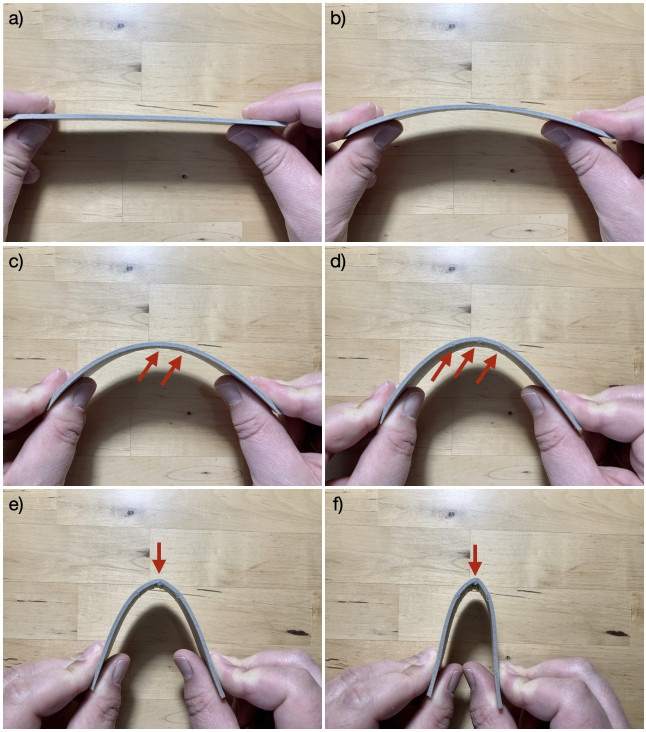
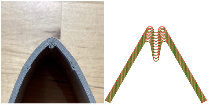
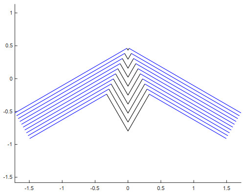
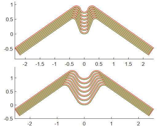
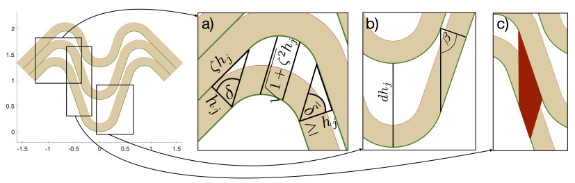
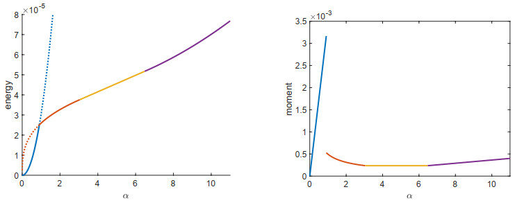
We develop and analyze a variational model for laminated paperboard. The model consists of a number of elastic sheets of a given thickness, which – at the expense of an energy per unit area – may delaminate. By providing an explicit construction for possible admissible deformations subject to boundary conditions that introduce a single bend, we discover a rich variety of energetic regimes. The regimes correspond to the experimentally observed: initial purely elastic response for small bending angle and the formation of a localized inelastic, delaminated hinge once the angle reaches a critical value. Our scaling upper bound then suggests the occurrence of several additional regimes as the angle increases. The upper bounds for the energy are partially matched by scaling lower bounds.
Citation: Sergio Conti, Patrick Dondl, Julia Orlik. Variational modeling of paperboard delamination under bending[J]. Mathematics in Engineering, 2023, 5(2): 1-28. doi: 10.3934/mine.2023039
We develop and analyze a variational model for laminated paperboard. The model consists of a number of elastic sheets of a given thickness, which – at the expense of an energy per unit area – may delaminate. By providing an explicit construction for possible admissible deformations subject to boundary conditions that introduce a single bend, we discover a rich variety of energetic regimes. The regimes correspond to the experimentally observed: initial purely elastic response for small bending angle and the formation of a localized inelastic, delaminated hinge once the angle reaches a critical value. Our scaling upper bound then suggests the occurrence of several additional regimes as the angle increases. The upper bounds for the energy are partially matched by scaling lower bounds.

| [1] | L. Ambrosio, N. Fusco, D. Pallara, Functions of bounded variation and free discontinuity problems, New York: The Clarendon Press, Oxford University Press, 2000. |
| [2] | S. S. Antman, Nonlinear problems of elasticity, New York: Springer, 2005. https://doi.org/10.1007/0-387-27649-1 |
| [3] | B. Audoly, Y. Pomeau, Elasticity and geometry: From hair curls to the non-linear response of shells, Oxford: Oxford University Press, 2010. |
| [4] |
L. A. A. Beex, R. H. J. Peerlings, An experimental and computational study of laminated paperboard creasing and folding, Int. J. Solids Struct., 46 (2009), 4192–4207. https://doi.org/10.1016/j.ijsolstr.2009.08.012 doi: 10.1016/j.ijsolstr.2009.08.012

|
| [5] |
L. A. A. Beex, R. H. J. Peerlings, On the influence of delamination on laminated paperboard creasing and folding, Phil. Trans. R. Soc. A, 370 (2012), 1912–1924. https://doi.org/10.1098/rsta.2011.0408 doi: 10.1098/rsta.2011.0408
|
| [6] |
H. Ben Belgacem, S. Conti, A. DeSimone, S. Müller, Rigorous bounds for the Föppl-von Kármán theory of isotropically compressed plates, J. Nonlinear Sci., 10 (2000), 661–683. https://doi.org/10.1007/s003320010007 doi: 10.1007/s003320010007
|
| [7] |
B. Bourdin, G. A. Francfort, J.-J. Marigo, The variational approach to fracture, J. Elasticity, 91 (2008), 5–148. https://doi.org/10.1007/s10659-007-9107-3 doi: 10.1007/s10659-007-9107-3
|
| [8] |
D. P. Bourne, S. Conti, S. Müller, Energy bounds for a compressed elastic film on a substrate, J. Nonlinear Sci., 27 (2017), 453–494. https://doi.org/10.1007/s00332-016-9339-0 doi: 10.1007/s00332-016-9339-0
|
| [9] |
S. Conti, F. Maggi, Confining thin elastic sheets and folding paper, Arch. Rational Mech. Anal., 187 (2008), 1–48. https://doi.org/10.1007/s00205-007-0076-2 doi: 10.1007/s00205-007-0076-2
|
| [10] |
G. Friesecke, R. D. James, S. Müller, A theorem on geometric rigidity and the derivation of nonlinear plate theory from three-dimensional elasticity, Commun. Pure Appl. Math., 55 (2002), 1461–1506. https://doi.org/10.1002/cpa.10048 doi: 10.1002/cpa.10048
|
| [11] | H. Huang, Numerical and experimental investigation of paperboard creasing and folding, PhD thesis, KTH Royal Institute of Technology, 2011. |
| [12] |
W. Jin, P. Sternberg, Energy estimates of the von Kármán model of thin-film blistering, J. Math. Phys., 42 (2001), 192–199. https://doi.org/10.1063/1.1316058 doi: 10.1063/1.1316058
|
| [13] | M. Klingenberg, A. Boldizar, K. Hofer, Mechanical properties of paperboard with a needled middle layer, Cell. Chem. Technol., 52 (2018), 89–97. |
| [14] |
R. V. Kohn, S. Müller, Surface energy and microstructure in coherent phase transitions, Commun. Pure Appl. Math., 47 (1994), 405–435. https://doi.org/10.1002/cpa.3160470402 doi: 10.1002/cpa.3160470402
|
| [15] | B. Lawn, Fracture of brittle solids, Cambridge: Cambridge University Press, 1993. https://doi.org/10.1017/CBO9780511623127 |
| [16] |
M. Lecumberry, S. Müller, Stability of slender bodies under compression and validity of the von Kármán theory, Arch. Rational Mech. Anal., 193 (2009), 255–310. https://doi.org/10.1007/s00205-009-0232-y doi: 10.1007/s00205-009-0232-y
|
| [17] | H. LeDret, A. Raoult, The nonlinear membrane model as a variational limit of nonlinear three-dimensional elasticity, J. Math. Pure. Appl., 73 (1995), 549–578. |
| [18] |
E. Linvill, M. Wallmeier, S. Östlund, A constitutive model for paperboard including wrinkle prediction and post-wrinkle behavior applied to deep drawing, Int. J. Solids Struct., 117 (2017), 143–158. https://doi.org/10.1016/j.ijsolstr.2017.03.029 doi: 10.1016/j.ijsolstr.2017.03.029
|
| [19] |
A. E. Lobkovsky, S. Gentges, H. Li, D. Morse, T. A. Witten, Scaling properties of stretching ridges in a crumpled elastic sheet, Science, 270 (1995), 1482–1485. https://doi.org/10.1126/science.270.5241.1482 doi: 10.1126/science.270.5241.1482
|
| [20] |
J. Orlik, Homogenization of strength, fatigue and creep durability of composites with near periodic structure, Math. Mod. Meth. Appl. Sci., 15 (2005), 1329–1347. https://doi.org/10.1142/S0218202505000807 doi: 10.1142/S0218202505000807
|
| [21] | S. Östlund, Three-dimensional deformation and damage mechanisms in forming of advanced structures in paper, In: Advances in pulp and paper research, Trans. of the XVIth Fund. Res. Symp. Oxford, 2017,489–594. |
| [22] |
J.-W. Simon, A review of recent trends and challenges in computational modeling of paper and paperboard at different scales, Arch. Computat. Methods Eng., 28 (2021), 2409–2428. https://doi.org/10.1007/s11831-020-09460-y doi: 10.1007/s11831-020-09460-y
|
| [23] |
S. C. Venkataramani, Lower bounds for the energy in a crumpled elastic sheet – a minimal ridge, Nonlinearity, 17 (2004), 301–312. https://doi.org/10.1088/0951-7715/17/1/017 doi: 10.1088/0951-7715/17/1/017
|
Figures(6)

Sergio Conti, Patrick Dondl, Julia Orlik. Variational modeling of paperboard delamination under bending[J]. Mathematics in Engineering, 2023, 5(2): 1-28. doi: 10.3934/mine.2023039


 DownLoad: