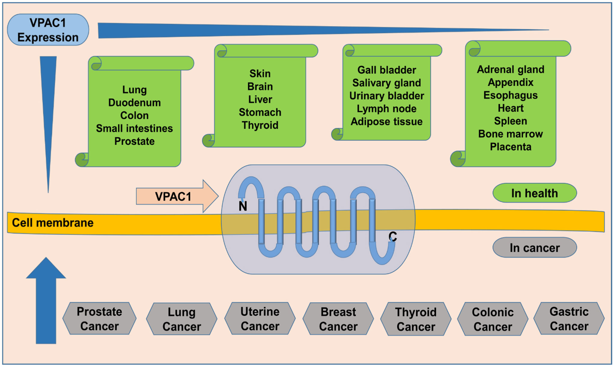
Prostate cancer is ranked as the fourth most prevalent cancer commonly diagnosed among males over 40 years of age, according to the WHO Cancer Fact Sheet 2020, and it is additionally a leading cause of cancer mortality among males. The incidence of prostate cancer and mortality varied significantly across the globe. Diagnosis of prostate cancer hinders easier management of cases, and prostate-specific antigen (PSA) use for screening of prostate cancer has poor specificity and sensitivity, thereby yielding overdiagnosis and unnecessary biopsies. Radiologically guided (ultrasound/MRI) prostate biopsy, considered the gold standard, is invasive and can miss a significant number of metastatic cancers. Even though mild, other prostate biopsy complications occur on a large scale, and few severe ones are often recorded. Scientists intensify their search for biomarker(s) for non-invasive diagnosis of prostate cancer using proteomics, metabolomics, genomics, and bioinformatics—urinary biomarkers were uniquely on the lookout. Vasoactive intestinal peptide (VIP)/pituitary adenylate cyclase-activating peptide (PACAP) receptor 1 (VPAC1), which is overexpressed (a thousandfold) in prostate cancer at the onset of oncogenesis and is excreted in the urine on tumor cells, is a contender in the prostate cancer biomarker quest. VPAC1 is ubiquitous, expressed by normal and malignant cells, and interwoven in their cell membranes. Therefore, using urine samples limits the possibility of making the wrong diagnosis, since VPAC1 is not normally excreted in the urine. Nevertheless, studying transmembrane receptors is intricate. However, producing monoclonal antibodies against the N-terminal end of VPAC1 can provide a promising target for designing a non-invasive diagnostic assay for early detection of prostate cancer using a urine sample.
Citation: Mansur Aliyu, Ali Akbar Saboor-Yaraghi, Shima Nejati, Behrouz Robat-Jazi. Urinary VPAC1: A potential biomarker in prostate cancer[J]. AIMS Allergy and Immunology, 2022, 6(2): 42-63. doi: 10.3934/Allergy.2022006
Prostate cancer is ranked as the fourth most prevalent cancer commonly diagnosed among males over 40 years of age, according to the WHO Cancer Fact Sheet 2020, and it is additionally a leading cause of cancer mortality among males. The incidence of prostate cancer and mortality varied significantly across the globe. Diagnosis of prostate cancer hinders easier management of cases, and prostate-specific antigen (PSA) use for screening of prostate cancer has poor specificity and sensitivity, thereby yielding overdiagnosis and unnecessary biopsies. Radiologically guided (ultrasound/MRI) prostate biopsy, considered the gold standard, is invasive and can miss a significant number of metastatic cancers. Even though mild, other prostate biopsy complications occur on a large scale, and few severe ones are often recorded. Scientists intensify their search for biomarker(s) for non-invasive diagnosis of prostate cancer using proteomics, metabolomics, genomics, and bioinformatics—urinary biomarkers were uniquely on the lookout. Vasoactive intestinal peptide (VIP)/pituitary adenylate cyclase-activating peptide (PACAP) receptor 1 (VPAC1), which is overexpressed (a thousandfold) in prostate cancer at the onset of oncogenesis and is excreted in the urine on tumor cells, is a contender in the prostate cancer biomarker quest. VPAC1 is ubiquitous, expressed by normal and malignant cells, and interwoven in their cell membranes. Therefore, using urine samples limits the possibility of making the wrong diagnosis, since VPAC1 is not normally excreted in the urine. Nevertheless, studying transmembrane receptors is intricate. However, producing monoclonal antibodies against the N-terminal end of VPAC1 can provide a promising target for designing a non-invasive diagnostic assay for early detection of prostate cancer using a urine sample.
prostate-specific antigen
vasoactive intestinal peptide
pituitary adenylate cyclase-activating peptide
VIP/PACAP receptor 1
age-standardized rate
benign prostatic hypertrophy
5α-dihydrotestosterone
quantitative reverse transcription polymerase chain reaction
magnetic resonance imaging
multiparametric MRI
dynamic contrast-enhanced MRI
diffusion-weighted imaging MRI
trans-rectal ultrasound scan
enzyme-linked immunosorbent assay
prostate cancer antigen 3
transmembrane protease serine 2
glutathione S-transferase P1
digital rectal examination
area under the curve
hepatocyte growth factor
insulin-like growth factor binding protein 3
Plasma osteopontin
lymph node carcinoma of the prostate
G protein-coupled receptors
receptor activity modifying proteins
seven-transmembrane domain
extracellular domain
Chinese hamster ovary
TATA-box binding protein
cyclooxygenase-2
metalloproteinase 9
urokinase plasminogen activator
uPA receptor
4,6-diamidino-2-phenylindole
adenylyl cyclase
cAMP response element-binding protein
phosphokinase A
inducible nitric oxide synthase
CREB binding protein
nuclear factor-κβ
extracellular signal-regulated kinase
MAP/ERK kinase (MEK) kinase 1
IFN regulatory factor-1
inhibitory κβ kinase
bombesin-like peptides
gastrin-releasing peptide receptor
phospholipase C
diacylglycerol
1,4,5-triphosphate
protein kinase C
mitogen-activated protein kinase
mitogen-activated protein kinase kinase
ETS like-1 protein
serum response element

| [1] |
Kimura T, Egawa S (2018) Epidemiology of prostate cancer in Asian countries. Int J Urol 25: 524-531. https://doi.org/10.1111/iju.13593 
|
| [2] |
Pernar CH, Ebot EM, Wilson KM, et al. (2018) The epidemiology of prostate cancer. Cold Spring Harbor Perspect Med 8: a030361-a030380. https://doi.org/10.1101/cshperspect.a030361
|
| [3] |
Adeloye D, David RA, Aderemi AV, et al. (2016) An estimate of the incidence of prostate cancer in Africa: A systematic review and meta-analysis. PLoS One 11: e0153496. https://doi.org/10.1371/journal.pone.0153496
|
| [4] |
Kang DY, Li HJ (2015) The effect of testosterone replacement therapy on prostate-specific antigen (PSA) levels in men being treated for hypogonadism: a systematic review and meta-analysis. Medicine 94: e410-e418. https://doi.org/10.1097/MD.0000000000000410
|
| [5] |
Ferlay J, Colombet M, Soerjomataram I, et al. (2019) Estimating the global cancer incidence and mortality in 2018: GLOBOCAN sources and methods. Int J Cancer 144: 1941-1953. https://doi.org/10.1002/ijc.31937
|
| [6] | (2018) World Health OrganisationCancer Fact Sheets. WHO. Available from: https://www.who.int/news-room/fact-sheets/detail/cancer |
| [7] |
Taitt HE (2018) Global trends and prostate cancer: a review of incidence, detection, and mortality as influenced by race, ethnicity, and geographic location. Am J Mens Health 12: 1807-1823. https://doi.org/10.1177/1557988318798279
|
| [8] |
Campi R, Brookman-May SD, Subiela Henriquez JD, et al. (2018) Impact of metabolic diseases, drugs, and dietary factors on prostate cancer risk, recurrence, and survival: A systematic review by the European Association of Urology Section of Oncological Urology. Eur Urol Focus 5: 1029-1057. https://doi.org/10.1016/j.euf.2018.04.001
|
| [9] |
Miah S, Catto J (2014) BPH and prostate cancer risk. Indian J Urol 30: 214-218. https://doi.org/10.4103/0970-1591.126909
|
| [10] |
Fernández-Martínez AB, Bajo AM, Arenas ML, et al. (2010) Vasoactive intestinal peptide (VIP) induces malignant transformation of the human prostate epithelial cell line RWPE-1. Cancer Lett 299: 11-21. https://doi.org/10.1016/j.canlet.2010.07.019
|
| [11] |
Boyle P, Koechlin A, Bota M, et al. (2016) Endogenous and exogenous testosterone and the risk of prostate cancer and increased prostate-specific antigen (PSA) level: a meta-analysis. BJU Int 118: 731-741. https://doi.org/10.1111/bju.13417
|
| [12] |
Tan ME, Li J, Xu HE, et al. (2015) Androgen receptor: structure, role in prostate cancer and drug discovery. Acta Pharmacol Sin 36: 3-23. https://doi.org/10.1038/aps.2014.18
|
| [13] |
Lee YJ, Park JE, Jeon BR, et al. (2013) Is prostate-specific antigen effective for population screening of prostate cancer? A systematic review. Ann Lab Med 33: 233-241. https://doi.org/10.3343/alm.2013.33.4.233
|
| [14] |
Negoita S, Feuer EJ, Mariotto A, et al. (2018) Annual report to the nation on the status of cancer, part II: Recent changes in prostate cancer trends and disease characteristics. Cancer 124: 2801-2814. https://doi.org/10.1002/cncr.31549
|
| [15] |
Zhang K, Aruva MR, Shanthly N, et al. (2008) PET imaging of VPAC1 expression in experimental and spontaneous prostate cancer. J Nucl Med 49: 112-121. https://doi.org/10.2967/jnumed.107.043703
|
| [16] |
Litwin MS, Tan HJ (2017) The diagnosis and treatment of prostate cancer: a review. JAMA 317: 2532-2542. https://doi.org/10.1001/jama.2017.7248
|
| [17] |
Renard-Penna R, Cancel-Tassin G, Comperat E, et al. (2015) Functional magnetic resonance imaging and molecular pathology at the crossroad of the management of early prostate cancer. World J Urol 33: 929-936. https://doi.org/10.1007/s00345-015-1570-z
|
| [18] |
Ahmed HU, Bosaily ESA, Brown LC, et al. (2017) Diagnostic accuracy of multi-parametric MRI and TRUS biopsy in prostate cancer (PROMIS): a paired validating confirmatory study. Lancet 389: 815-822. https://doi.org/10.1016/S0140-6736(16)32401-1
|
| [19] | Boesen L (2017) Multiparametric MRI in detection and staging of prostate cancer. Dan Med J 64: B5327. |
| [20] | Sosnowski R, Zagrodzka M, Borkowski T (2016) The limitations of multiparametric magnetic resonance imaging also must be borne in mind. Cent Eur J Urol 69: 22-23. https://doi.org/10.5173/ceju.2016.e113 |
| [21] |
Saini S (2016) PSA and beyond: alternative prostate cancer biomarkers. Cell Oncol 39: 97-106. https://doi.org/10.1007/s13402-016-0268-6
|
| [22] |
Zhao L, Yu N, Guo T, et al. (2014) Tissue biomarkers for prognosis of prostate cancer: A systematic review and meta-analysis. Cancer Epidem Biomar 23: 1047-1054. https://doi.org/10.1158/1055-9965.EPI-13-0696
|
| [23] |
Jedinak A, Loughlin KR, Moses MA (2018) Approaches to the discovery of non-invasive urinary biomarkers of prostate cancer. Oncotarget 9: 32534-32550. https://doi.org/10.18632/oncotarget.25946
|
| [24] |
Wu D, Ni J, Beretov J, et al. (2017) Urinary biomarkers in prostate cancer detection and monitoring progression. Crit Rev Oncol Hemat 118: 15-26. https://doi.org/10.1016/j.critrevonc.2017.08.002
|
| [25] |
Tosoian JJ, Ross AE, Sokoll LJ, et al. (2016) Urinary biomarkers for prostate cancer. Urol Clin N Am 43: 17-38. https://doi.org/10.1016/j.ucl.2015.08.003
|
| [26] |
Luo Y, Gou X, Huang P, et al. (2014) The PCA3 test for guiding repeat biopsy of prostate cancer and its cut-off score: a systematic review and meta-analysis. Asian J Androl 16: 487-492. https://doi.org/10.4103/1008-682X.125390
|
| [27] |
Dijkstra S, Mulders PF, Schalken JA (2014) Clinical use of novel urine and blood based prostate cancer biomarkers: a review. Clin Biochem 47: 889-896. https://doi.org/10.1016/j.clinbiochem.2013.10.023
|
| [28] |
Larsen LK, Jakobsen JS, Abdul-Al A, et al. (2018) Noninvasive detection of high-grade prostate cancer by DNA methylation analysis of urine cells captured by microfiltration. J Uroly 200: 749-757. https://doi.org/10.1016/j.juro.2018.04.067
|
| [29] |
Ratz L, Laible M, Kacprzyk LA, et al. (2017) TMPRSS2:ERG gene fusion variants induce TGF-β signaling and epithelial to mesenchymal transition in human prostate cancer cells. Oncotarget 8: 25115-25130. https://doi.org/10.18632/oncotarget.15931
|
| [30] |
Sequeiros T, Bastarós JM, Sánchez M, et al. (2015) Urinary biomarkers for the detection of prostate cancer in patients with high-grade prostatic intraepithelial neoplasia. Prostate 75: 1102-1113. https://doi.org/10.1002/pros.22995
|
| [31] |
Mengual L, Lozano JJ, Ingelmo-Torres M, et al. (2016) Using gene expression from urine sediment to diagnose prostate cancer: development of a new multiplex mRNA urine test and validation of current biomarkers. BMC Cancer 16: 76. https://doi.org/10.1186/s12885-016-2127-2
|
| [32] |
Fryczkowski M, Bułdak R, Hejmo T, et al. (2018) Circulating levels of omentin, leptin, VEGF, and HGF and their clinical relevance with PSA marker in prostate cancer. Dis Markers 2018: 3852401. https://doi.org/10.1155/2018/3852401
|
| [33] | Dheeraj A, Tailor D, Deep G, et al. (2018) Insulin-like Growth Factor Binding Protein-3 (IGFBP-3) regulates mitochondrial dynamics, EMT, and angiogenesis in progression of prostate cancer. Cancer Res 78: 1095. https://doi.org/10.1158/1538-7445.AM2018-1095 |
| [34] | Wisniewski T, Zyromska A, Makarewicz R, et al. (2019) Osteopontin and angiogenic factors as new biomarkers of prostate cancer. Urol J 16: 134-140. |
| [35] |
Prager AJ, Peng CR, Lita E, et al. (2013) Urinary aHGF, IGFBP3, and OPN as diagnostic and prognostic biomarkers for prostate cancer. Biomarkers Med 7: 831-841. https://doi.org/10.2217/bmm.13.112
|
| [36] |
Rivnyak A, Kiss P, Tamas A, et al. (2018) Review on PACAP-induced transcriptomic and proteomic changes in neuronal development and repair. Int J Mol Sci 19: 1020. https://doi.org/10.3390/ijms19041020
|
| [37] |
Ashina M, Martelletti P (2018) Pituitary adenylate-cyclase-activating polypeptide (PACAP): another novel target for treatment of primary headaches?. J Headache Pain 19: 33. https://doi.org/10.1186/s10194-018-0860-4
|
| [38] |
Johnson GC, Parsons R, May V, et al. (2020) The role of pituitary adenylate cyclase-activating polypeptide (PACAP) signaling in the hippocampal dentate gyrus. Front Cell Neurosci 14: 111. https://doi.org/10.3389/fncel.2020.00111
|
| [39] |
Hirabayashi T, Nakamachi T, Shioda S (2018) Discovery of PACAP and its receptors in the brain. J Headache Pain 19: 28. https://doi.org/10.1186/s10194-018-0855-1
|
| [40] |
Leyton J, Coelho T, Coy D, et al. (1998) PACAP (6–38) inhibits the growth of prostate cancer cells. Cancer Lett 125: 131-139. https://doi.org/10.1016/S0304-3835(97)00525-9
|
| [41] |
Derand R, Montoni A, Bulteau-Pignoux L, et al. (2004) Activation of VPAC1 receptors by VIP and PACAP-27 in human bronchial epithelial cells induces CFTR-dependent chloride secretion. Brit J Pharmacol 141: 698-708. https://doi.org/10.1038/sj.bjp.0705597
|
| [42] |
Couvineau A, Ceraudo E, Tan YV, et al. (2012) The VPAC1 receptor: structure and function of a class B GPCR prototype. Front Endocrinol 3: 139. https://doi.org/10.3389/fendo.2012.00139
|
| [43] |
Couvineau A, Tan YV, Ceraudo E, et al. (2013) Strategies for studying the ligand-binding site of GPCRs: Photoaffinity labeling of the VPAC1 receptor, a prototype of class B GPCRs. Method Enzymol 520: 219-237. https://doi.org/10.1016/B978-0-12-391861-1.00010-1
|
| [44] |
Starr CG, Maderdrut JL, He J, et al. (2018) Pituitary adenylate cyclase-activating polypeptide is a potent broad-spectrum antimicrobial peptide: Structure-activity relationships. Peptides 104: 35-40. https://doi.org/10.1016/j.peptides.2018.04.006
|
| [45] |
Jayawardena D, Guzman G, Gill RK, et al. (2017) Expression and localization of VPAC1, the major receptor of vasoactive intestinal peptide along the length of the intestine. Am J Physiol-Gastr L 313: G16-G25. https://doi.org/10.1152/ajpgi.00081.2017
|
| [46] |
Dorsam GP, Benton K, Failing J, et al. (2011) Vasoactive intestinal peptide signaling axis in human leukemia. World J Biol Chem 2: 146-160. https://doi.org/10.4331/wjbc.v2.i6.146
|
| [47] |
Garcı́a-Fernández MO, Solano RM, Carmena MJ, et al. (2003) Expression of functional PACAP/VIP receptors in human prostate cancer and healthy tissue. Peptides 24: 893-902. https://doi.org/10.1016/S0196-9781(03)00162-1
|
| [48] |
Moretti C, Mammi C, Frajese GV, et al. (2006) PACAP and type I PACAP receptors in human prostate cancer tissue. Ann NY Acad Sci 1070: 440-449. https://doi.org/10.1196/annals.1317.059
|
| [49] |
Tamas A, Javorhazy A, Reglodi D, et al. (2016) Examination of PACAP-like immunoreactivity in urogenital tumor samples. J Mol Neurosci 59: 177-183. https://doi.org/10.1007/s12031-015-0652-0
|
| [50] |
Ibrahim H, Barrow P, Foster N (2011) Transcriptional modulation by VIP: a rational target against inflammatory disease. Clin Epigenet 2: 213-222. https://doi.org/10.1007/s13148-011-0036-4
|
| [51] |
Gomariz RP, Juarranz Y, Carrión M, et al. (2019) An overview of VPAC receptors in rheumatoid arthritis: biological role and clinical significance. Front Endocrinol 10: 729. https://doi.org/10.3389/fendo.2019.00729
|
| [52] |
Couvineau A, Laburthe M (2012) VPAC receptors: structure, molecular pharmacology, and interaction with accessory proteins. Brit J Pharmacol 166: 42-50. https://doi.org/10.1111/j.1476-5381.2011.01676.x
|
| [53] |
Tripathi S, Trabulsi EJ, Gomella L, et al. (2016) VPAC1 targeted (64)Cu-TP3805 positron emission tomography imaging of prostate cancer: preliminary evaluation in man. Urology 88: 111-118. https://doi.org/10.1016/j.urology.2015.10.012
|
| [54] |
Arms L, Vizzard MA (2011) Neuropeptides in lower urinary tract function. Handbook of Experimental Pharmacology : 395-423. https://doi.org/10.1007/978-3-642-16499-6_19
|
| [55] |
Inbal U, Alexandraki K, Grozinsky-Glasberg S (2018) Gastrointestinal hormones in cancer. Encyclopedia of Endocrine Diseases . Oxford: Academic Press 579-586. https://doi.org/10.1016/B978-0-12-801238-3.95875-6
|
| [56] |
Tang B, Yong X, Xie R, et al. (2014) Vasoactive intestinal peptide receptor-based imaging and treatment of tumors (Review). Int J Oncol 44: 1023-1031. https://doi.org/10.3892/ijo.2014.2276
|
| [57] |
Reubi JC (2000) In vitro evaluation of VIP/PACAP receptors in healthy and diseased human tissues: clinical implications. Ann NY Acad Sci 921: 1-25. https://doi.org/10.1111/j.1749-6632.2000.tb06946.x
|
| [58] | Thakur ML (2016) Targeting VPAC1 genomic receptors for optical imaging of lung cancer. Eur J Nucl Med Mol Imaging 43: S662-S663. |
| [59] |
Tang B, Wu J, Zhu MX, et al. (2019) VPAC1 couples with TRPV4 channel to promote calcium-dependent gastric cancer progression via a novel autocrine mechanism. Oncogene 38: 3946-3961. https://doi.org/10.1038/s41388-019-0709-6
|
| [60] |
Truong H, Gomella LG, Thakur ML, et al. (2018) VPAC1-targeted PET/CT scan: improved molecular imaging for the diagnosis of prostate cancer using a novel cell surface antigen. World J Urol 36: 719-726. https://doi.org/10.1007/s00345-018-2263-1
|
| [61] |
Liu S, Zeng Y, Li Y, et al. (2014) VPAC1 overexpression is associated with poor differentiation in colon cancer. Tumour Biol 35: 6397-6404. https://doi.org/10.1007/s13277-014-1852-x
|
| [62] | Tang B, Xie R, Xiao YF, et al. (2017) VIP promotes gastric cancer progression via the VPAC1/TRPV4/Ca2+ signaling pathway. J Dig Dis 152: S836. https://doi.org/10.1016/S0016-5085(17)32886-X |
| [63] | Tripathi S, Trabulsi E, Kumar P, et al. (2015) VPAC1 targeted detection of genitourinary cancer: A urinary assay. J Nuclear Med 56: 388. |
| [64] |
Delgado M, Pozo D, Ganea D (2004) The significance of vasoactive intestinal peptide in immunomodulation. Pharmacol Rev 56: 249-290. https://doi.org/10.1124/pr.56.2.7
|
| [65] |
Ganea D, Hooper KM, Kong W (2015) The neuropeptide vasoactive intestinal peptide: direct effects on immune cells and involvement in inflammatory and autoimmune diseases. Acta Physiol 213: 442-452. https://doi.org/10.1111/apha.12427
|
| [66] |
Wu F, Song G, de Graaf C, et al. (2017) Structure and function of peptide-binding G protein-coupled receptors. J Mol Biol 429: 2726-2745. https://doi.org/10.1016/j.jmb.2017.06.022
|
| [67] |
Moody TW (2019) Peptide receptors as cancer drug targets. Ann NY Acad Sci 1455: 141-148. https://doi.org/10.1111/nyas.14100
|
| [68] |
Latek D, Langer I, Krzysko K, et al. (2019) A molecular dynamics study of vasoactive intestinal peptide receptor 1 and the basis of its therapeutic antagonism. Int J Mol Sci 20: 4348-4369. https://doi.org/10.3390/ijms20184348
|
| [69] |
Langer I (2012) Conformational switches in the VPAC1 receptor. Brit J Pharmacol 166: 79-84. https://doi.org/10.1111/j.1476-5381.2011.01616.x
|
| [70] |
Santos R, Ursu O, Gaulton A, et al. (2017) A comprehensive map of molecular drug targets. Nat Rev Drug Discov 16: 19-34. https://doi.org/10.1038/nrd.2016.230
|
| [71] |
de Graaf C, Song G, Cao C, et al. (2017) Extending the structural view of class B GPCRs. Trends Biochem Sci 42: 946-960. https://doi.org/10.1016/j.tibs.2017.10.003
|
| [72] |
Solano RM, Langer I, Perret J, et al. (2001) Two basic residues of the h-VPAC1 receptor second transmembrane helix are essential for ligand binding and signal transduction. J Biol Chem 276: 1084-1088. https://doi.org/10.1074/jbc.M007696200
|
| [73] |
Jazayeri A, Doré AS, Lamb D, et al. (2016) Extra-helical binding site of a glucagon receptor antagonist. Nature 533: 274. https://doi.org/10.1038/nature17414
|
| [74] |
Parthier C, Reedtz-Runge S, Rudolph R, et al. (2009) Passing the baton in class B GPCRs: peptide hormone activation via helix induction?. Trends Biochem Sci 34: 303-310. https://doi.org/10.1016/j.tibs.2009.02.004
|
| [75] |
Ceraudo E, Hierso R, Tan YV, et al. (2012) Spatial proximity between the VPAC1 receptor and the amino terminus of agonist and antagonist peptides reveals distinct sites of interaction. FASEB J 26: 2060-2071. https://doi.org/10.1096/fj.11-196444
|
| [76] |
Hutchings CJ, Koglin M, Olson WC, et al. (2017) Opportunities for therapeutic antibodies directed at G-protein-coupled receptors. Nat Rev Drug Discov 16: 787-810. https://doi.org/10.1038/nrd.2017.91
|
| [77] |
Peyrassol X, Laeremans T, Lahura V, et al. (2018) Development by genetic immunization of monovalent antibodies against human vasoactive intestinal peptide receptor 1 (VPAC1), new innovative, and versatile tools to study VPAC1 receptor function. Front Endocrinol 9: 153. https://doi.org/10.3389/fendo.2018.00153
|
| [78] |
Freson K, Peeters K, De Vos R, et al. (2008) PACAP and its receptor VPAC1 regulate megakaryocyte maturation: therapeutic implications. Blood 111: 1885-1893. https://doi.org/10.1182/blood-2007-06-098558
|
| [79] |
Hermann RJ, Van der Steen T, Vomhof-Dekrey EE, et al. (2012) Characterization and use of a rabbit-anti-mouse VPAC1 antibody by flow cytometry. J Immunol Methods 376: 20-31. https://doi.org/10.1016/j.jim.2011.10.009
|
| [80] |
Langlet C, Langer I, Vertongen P, et al. (2005) Contribution of the carboxyl terminus of the VPAC1 receptor to agonist-induced receptor phosphorylation, internalization, and recycling. J Biol Chem 280: 28034-28043. https://doi.org/10.1074/jbc.M500449200
|
| [81] |
Ramos-Álvarez I, Mantey SA, Nakamura T, et al. (2015) A structure-function study of PACAP using conformationally restricted analogs: Identification of PAC1 receptor-selective PACAP agonists. Peptides 66: 26-42. https://doi.org/10.1016/j.peptides.2015.01.009
|
| [82] |
Van Rampelbergh J, Juarranz MG, Perret J, et al. (2000) Characterization of a novel VPAC1 selective agonist and identification of the receptor domains implicated in the carboxyl-terminal peptide recognition. Brit J Pharmacol 130: 819-826. https://doi.org/10.1038/sj.bjp.0703384
|
| [83] |
Dickson L, Aramori I, McCulloch J, et al. (2006) A systematic comparison of intracellular cyclic AMP and calcium signalling highlights complexities in human VPAC/PAC receptor pharmacology. Neuropharmacol 51: 1086-1098. https://doi.org/10.1016/j.neuropharm.2006.07.017
|
| [84] |
Moody TW, Nuche-Berenguer B, Jensen RT (2016) Vasoactive intestinal peptide/pituitary adenylate cyclase-activating polypeptide, and their receptors and cancer. Curr Opin Endocrinol 23: 38-47. https://doi.org/10.1097/MED.0000000000000218
|
| [85] |
Moody TW, Chan D, Fahrenkrug J, et al. (2003) Neuropeptides as autocrine growth factors in cancer cells. Curr Pharm Design 9: 495-509. https://doi.org/10.2174/1381612033391621
|
| [86] |
Fernández-Martínez AB, Carmena MJ, Bajo AM, et al. (2015) VIP induces NF-κB1-nuclear localisation through different signalling pathways in human tumour and non-tumour prostate cells. Cell Signal 27: 236-244. https://doi.org/10.1016/j.cellsig.2014.11.005
|
| [87] |
Iwasaki M, Akiba Y, Kaunitz JD (2019) Recent advances in vasoactive intestinal peptide physiology and pathophysiology: focus on the gastrointestinal system. F1000Research 8: 1629-1642. https://doi.org/10.12688/f1000research.18039.1
|
| [88] |
Langer I (2012) Mechanisms involved in VPAC receptors activation and regulation: lessons from pharmacological and mutagenesis studies. Front Endocrin 3: 129. https://doi.org/10.3389/fendo.2012.00129
|
| [89] |
Harmar AJ, Fahrenkrug J, Gozes I, et al. (2012) Pharmacology and functions of receptors for vasoactive intestinal peptide and pituitary adenylate cyclase—activating polypeptide: IUPHAR Review 1. Brit J Pharmacol 166: 4-17. https://doi.org/10.1111/j.1476-5381.2012.01871.x
|
| [90] |
Langer I, Robberecht P (2007) Molecular mechanisms involved in vasoactive intestinal peptide receptor activation and regulation: current knowledge, similarities to and differences from the A family of G-protein-coupled receptors. Biochem Soc Trans 35: 724-728. https://doi.org/10.1042/BST0350724
|
| [91] |
Igarashi H, Fujimori N, Ito T, et al. (2011) Vasoactive intestinal peptide (VIP) and VIP receptors-elucidation of structure and function for therapeutic applications. Int J Clin Med 2: 500-508. https://doi.org/10.4236/ijcm.2011.24084
|
| [92] |
Delgado M, Ganea D (2000) Inhibition of IFN-gamma-induced Janus kinase-1-STAT1 activation in macrophages by vasoactive intestinal peptide and pituitary adenylate cyclase-activating polypeptide. J Immunol 165: 3051-3057. https://doi.org/10.4049/jimmunol.165.6.3051
|
| [93] |
Smalley SGR, Barrow PA, Foster N (2009) Immunomodulation of innate immune responses by vasoactive intestinal peptide (VIP): its therapeutic potential in inflammatory disease. Clin Exp Immunol 157: 225-234. https://doi.org/10.1111/j.1365-2249.2009.03956.x
|
| [94] |
Shaywitz AJ, Greenberg ME (1999) CREB: a stimulus-induced transcription factor activated by a diverse array of extracellular signals. Annu Rev Biochem 68: 821-861. https://doi.org/10.1146/annurev.biochem.68.1.821
|
| [95] |
Delgado M, Ganea D (2001) Vasoactive intestinal peptide and pituitary adenylate cyclase-activating polypeptide inhibit nuclear factor-kappa B-dependent gene activation at multiple levels in the human monocytic cell line THP-1. J Biol Chem 276: 369-380. https://doi.org/10.1074/jbc.M006923200
|
| [96] |
Dickson L, Finlayson K (2009) VPAC and PAC receptors: From ligands to function. Pharmacol Therapeut 121: 294-316. https://doi.org/10.1016/j.pharmthera.2008.11.006
|
| [97] |
Laburthe M, Couvineau A, Tan V (2007) Class II G protein-coupled receptors for VIP and PACAP: Structure, models of activation and pharmacology. Peptides 28: 1631-1639. https://doi.org/10.1016/j.peptides.2007.04.026
|
| [98] |
Collado B, Sánchez MG, Díaz-Laviada I, et al. (2005) Vasoactive intestinal peptide (VIP) induces c-fos expression in LNCaP prostate cancer cells through a mechanism that involves Ca2+ signalling. Implications in angiogenesis and neuroendocrine differentiation. Biochim Biophys Acta Mol Cell Res 1744: 224-233. https://doi.org/10.1016/j.bbamcr.2005.04.009
|
| [99] |
Park MH, Hong JT (2016) Roles of NF-κB in cancer and inflammatory diseases and their therapeutic approaches. Cells 5: 15. https://doi.org/10.3390/cells5020015
|
| [100] |
Grosset AA, Ouellet V, Caron C, et al. (2019) Validation of the prognostic value of NF-κB p65 in prostate cancer: A retrospective study using a large multi-institutional cohort of the Canadian Prostate Cancer Biomarker Network. PLoS Med 16: e1002847. https://doi.org/10.1371/journal.pmed.1002847
|
| [101] |
Staal J, Beyaert R (2018) Inflammation and NF-κB signaling in prostate cancer: mechanisms and clinical implications. Cells 7: 122. https://doi.org/10.3390/cells7090122
|
| [102] |
Thomas-Jardin SE, Dahl H, Nawas AF, et al. (2020) NF-κB signaling promotes castration-resistant prostate cancer initiation and progression. Pharmacol Therapeut 211: 107538. https://doi.org/10.1016/j.pharmthera.2020.107538
|
| [103] |
Jain G, Cronauer MV, Schrader M, et al. (2012) NF-kappaB signaling in prostate cancer: a promising therapeutic target?. World J Urol 30: 303-310. https://doi.org/10.1007/s00345-011-0792-y
|
| [104] |
Moreno P, Ramos-Álvarez I, Moody TW, et al. (2016) Bombesin-related peptides/receptors and their promising therapeutic roles in cancer imaging, targeting, and treatment. Expert Opin Ther Targets 20: 1055-1073. https://doi.org/10.1517/14728222.2016.1164694
|
| [105] |
Ramos-Álvarez I, Moreno P, Mantey SA, et al. (2015) Insights into bombesin receptors and ligands: Highlighting recent advances. Peptides 72: 128-144. https://doi.org/10.1016/j.peptides.2015.04.026
|
| [106] |
Baratto L, Jadvar H, Iagaru A (2018) Prostate cancer theranostics targeting gastrin-releasing peptide receptors. Mol Imaging Biol 20: 501-509. https://doi.org/10.1007/s11307-017-1151-1
|
| [107] |
Moody TW, Ramos-Alvarez I, Jensen RT (2018) Neuropeptide G protein-coupled receptors as oncotargets. Front Endocrinol 9: 345-345. https://doi.org/10.3389/fendo.2018.00345
|
| [108] | Dai J, Shen R, Sumitomo M, et al. (2002) Synergistic activation of the androgen receptor by bombesin and low-dose androgen. Clin Cancer Res 8: 2399. |
| [109] |
Putney JW, Tomita T (2012) Phospholipase C signaling and calcium influx. Adv Biol Regul 52: 152-164. https://doi.org/10.1016/j.advenzreg.2011.09.005
|
| [110] |
Weber HC (2009) Regulation and signaling of human bombesin receptors and their biological effects. Curr Opin Endocrinol 16: 66-71. https://doi.org/10.1097/MED.0b013e32831cf5aa
|
| [111] |
Fujita K, Pavlovich CP, Netto GJ, et al. (2009) Specific detection of prostate cancer cells in urine by multiplex immunofluorescence cytology. Hum Pathol 40: 924-933. https://doi.org/10.1016/j.humpath.2009.01.004
|
| [112] |
Fujita K, Nonomura N (2018) Urinary biomarkers of prostate cancer. Int J Urol 25: 770-779. https://doi.org/10.1111/iju.13734
|
| [113] |
Wei JT (2015) Urinary biomarkers for prostate cancer. Curr Opin Urol 25: 77-82. https://doi.org/10.1097/MOU.0000000000000133
|
| [114] |
Trabulsi EJ, Tripathi SK, Gomella L, et al. (2017) Development of a voided urine assay for detecting prostate cancer non-invasively: a pilot study. BJU Int 119: 885-895. https://doi.org/10.1111/bju.13775
|
| [115] |
Trabulsi E, Tripathi S, Calvaresi A, et al. (2016) VPAC1 in shed urinary cells—A potential genitourinary cancer biomarker. J Urol 195: e12. https://doi.org/10.1016/j.juro.2016.02.1880
|
| [116] | Hoepel J (2021) Unraveling the mechanisms of antibody-dependent inflammation [PhD's thesis]. University of Amsterdam, Netherlands . |
| [117] |
Lagerström MC, Schiöth HB (2008) Structural diversity of G protein-coupled receptors and significance for drug discovery. Nat Rev Drug Discov 7: 339-357. https://doi.org/10.1038/nrd2518
|
| [118] |
Pediani JD, Ward RJ, Marsango S, et al. (2018) Spatial intensity distribution analysis: studies of G protein-coupled receptor oligomerisation. Trends Pharmacol Sci 39: 175-186. https://doi.org/10.1016/j.tips.2017.09.001
|
| [119] |
Hutchings CJ, Koglin M, Marshall FH (2010) Therapeutic antibodies directed at G protein-coupled receptors. mAbs 2: 594-606. https://doi.org/10.4161/mabs.2.6.13420
|
Figures(3)

Mansur Aliyu, Ali Akbar Saboor-Yaraghi, Shima Nejati, Behrouz Robat-Jazi. Urinary VPAC1: A potential biomarker in prostate cancer[J]. AIMS Allergy and Immunology, 2022, 6(2): 42-63. doi: 10.3934/Allergy.2022006


 DownLoad: