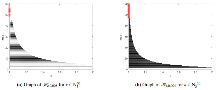
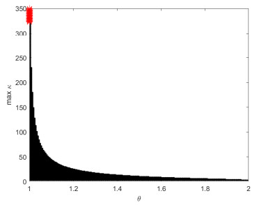
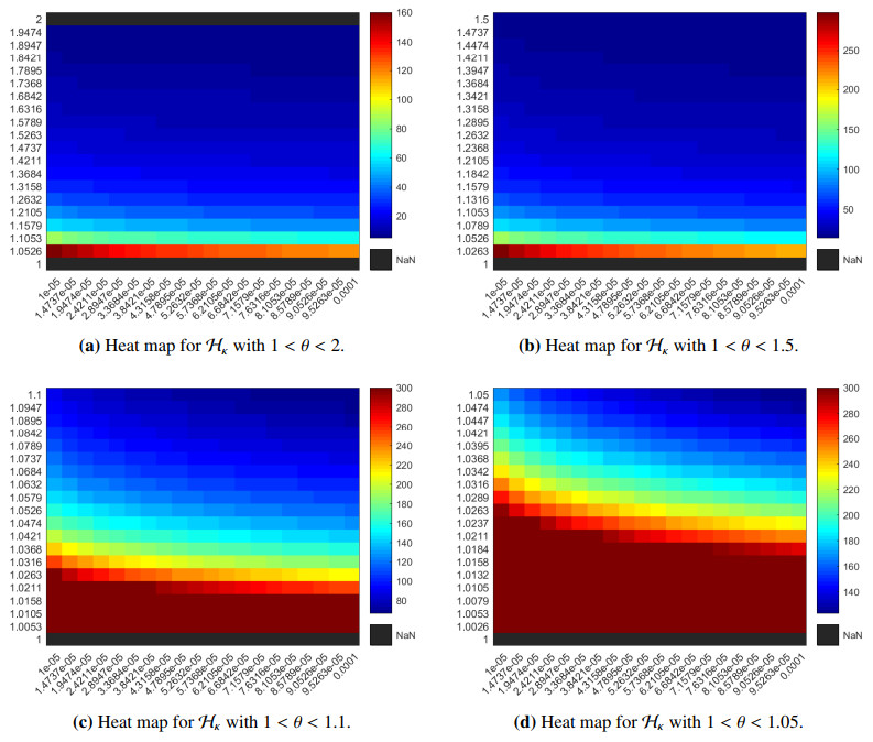
We study the monotonicity method to analyse nabla positivity for discrete fractional operators of Riemann-Liouville type based on exponential kernels, where $ \left({}_{{c_0}}^{C{F_R}}\nabla^{\theta} \mathtt{F}\right)(t) > -\epsilon\, \Lambda(\theta-1)\, \bigl(\nabla \mathtt{F}\bigr)(c_{0}+1) $ such that $ \bigl(\nabla \mathtt{F}\bigr)(c_{0}+1)\geq 0 $ and $ \epsilon > 0 $. Next, the positivity of the fully discrete fractional operator is analyzed, and the region of the solution is presented. Further, we consider numerical simulations to validate our theory. Finally, the region of the solution and the cardinality of the region are discussed via standard plots and heat map plots. The figures confirm the region of solutions for specific values of $ \epsilon $ and $ \theta $.
Citation: Pshtiwan Othman Mohammed, Donal O'Regan, Dumitru Baleanu, Y. S. Hamed, Ehab E. Elattar. Analytical results for positivity of discrete fractional operators with approximation of the domain of solutions[J]. Mathematical Biosciences and Engineering, 2022, 19(7): 7272-7283. doi: 10.3934/mbe.2022343
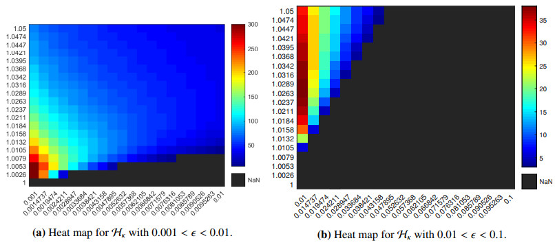
We study the monotonicity method to analyse nabla positivity for discrete fractional operators of Riemann-Liouville type based on exponential kernels, where $ \left({}_{{c_0}}^{C{F_R}}\nabla^{\theta} \mathtt{F}\right)(t) > -\epsilon\, \Lambda(\theta-1)\, \bigl(\nabla \mathtt{F}\bigr)(c_{0}+1) $ such that $ \bigl(\nabla \mathtt{F}\bigr)(c_{0}+1)\geq 0 $ and $ \epsilon > 0 $. Next, the positivity of the fully discrete fractional operator is analyzed, and the region of the solution is presented. Further, we consider numerical simulations to validate our theory. Finally, the region of the solution and the cardinality of the region are discussed via standard plots and heat map plots. The figures confirm the region of solutions for specific values of $ \epsilon $ and $ \theta $.

| [1] | C. Goodrich, A. C. Peterson, Discrete Fractional Calculus, Springer, Berlin, 2015. https://doi.org/10.1007/978-3-319-25562-0 |
| [2] |
T. Abdeljawad, D. Baleanu, On fractional derivatives with exponential kernel and their discrete versions, Rep. Math. Phys., 80 (2017), 11–27. https://doi.org/10.1016/S0034-4877(17)30059-9 doi: 10.1016/S0034-4877(17)30059-9

|
| [3] |
T. Abdeljawad, Q. M. Al-Mdallal, M. A. Hajji, Arbitrary order fractional difference operators with discrete exponential kernels and applications, Discrete Dyn. Nat. Soc., 2017 (2017). https://doi.org/10.1155/2017/4149320 doi: 10.1155/2017/4149320
|
| [4] |
T. Abdeljawad, On Riemann and Caputo fractional differences, Comput. Math. Appl., 62 (2011), 1602–1611. https://doi.org/10.1016/j.camwa.2011.03.036 doi: 10.1016/j.camwa.2011.03.036
|
| [5] |
T. Abdeljawad, Different type kernel $h$–fractional differences and their fractional $h$–sums, Chaos, Solitons Fractals, 116 (2018), 146–156. https://doi.org/10.1016/j.chaos.2018.09.022 doi: 10.1016/j.chaos.2018.09.022
|
| [6] |
P. O. Mohammed, T. Abdeljawad, Discrete generalized fractional operators defined using h-discrete Mittag-Leffler kernels and applications to AB fractional difference systems, Math. Methods Appl. Sci., (2020), 1–26, https://doi.org/10.1002/mma.7083 doi: 10.1002/mma.7083
|
| [7] |
G. C. Wu, M. K. Luo, L. L. Huang, S. Banerjee, Short memory fractional differential equations for new neural network and memristor design, Nonlinear Dyn., 100 (2020), 3611–3623. https://doi.org/10.1007/s11071-020-05572-z doi: 10.1007/s11071-020-05572-z
|
| [8] |
L. L. Huang, G. C. Wu, D. Baleanu, H. Y. Wang, Discrete fractional calculus for interval-valued systems, Fuzzy Sets Syst., 404 (2021), 141–158. https://doi.org/10.1016/j.fss.2020.04.008 doi: 10.1016/j.fss.2020.04.008
|
| [9] |
T. Abdeljawad, S. Banerjee, G. C. Wu, Discrete tempered fractional calculus for new chaotic systems with short memory and image encryption, Optik, 2018 (2020), 163698. https://doi.org/10.1016/j.ijleo.2019.163698 doi: 10.1016/j.ijleo.2019.163698
|
| [10] |
G. C. Wu, D. Baleanu, Discrete fractional logistic map and its chaos, Nonlinear Dyn., 75 (2014), 283–287. https://doi.org/10.1007/s11071-013-1065-7 doi: 10.1007/s11071-013-1065-7
|
| [11] |
R. Dahal, C. S. Goodrich, A monotonocity result for discrete fractional difference operators, Arch. Math., 102 (2014), 293–299. https://doi.org/10.1007/s00013-014-0620-x doi: 10.1007/s00013-014-0620-x
|
| [12] |
C. S. Goodrich, A convexity result for fractional differences, Appl. Math. Lett., 35 (2014), 158–162. https://doi.org/10.1016/j.aml.2014.04.013 doi: 10.1016/j.aml.2014.04.013
|
| [13] |
F. Atici, M. Uyanik, Analysis of discrete fractional operators, Appl. Anal. Discrete Math., 9 (2015), 139–149. https://doi.org/10.2298/AADM150218007A doi: 10.2298/AADM150218007A
|
| [14] |
P. O. Mohammed, O. Almutairi, R. P. Agarwal, Y. S. Hamed, On convexity, monotonicity and positivity analysis for discrete fractional operators defined using exponential kernels, Fractal Fractional, 6 (2022), 55. https://doi.org/10.3390/fractalfract6020055 doi: 10.3390/fractalfract6020055
|
| [15] |
T. Abdeljawad, D. Baleanu, Monotonicity analysis of a nabla discrete fractional operator with discrete Mittag-Leffler kernel, Chaos, Solitons Fractals, 102 (2017), 106–110. https://doi.org/10.1016/j.chaos.2017.04.006 doi: 10.1016/j.chaos.2017.04.006
|
| [16] |
P. O. Mohammed, C. S. Goodrich, A. B. Brzo, Y. S. Hamed, New classifications of monotonicity investigation for discrete operators with Mittag-Leffler kernel, Math. Biosci. Eng., 19 (2022), 4062–4074. https://doi.org/10.3934/mbe.2022186 doi: 10.3934/mbe.2022186
|
| [17] |
C. Goodrich, C. Lizama, Positivity, monotonicity, and convexity for convolution operators, Discrete Contin. Dyn. Syst., 40 (2020), 4961–4983. https://doi.org/10.3934/dcds.2020207 doi: 10.3934/dcds.2020207
|
| [18] |
C. S. Goodrich, B. Lyons, Positivity and monotonicity results for triple sequential fractional differences via convolution, Analysis, 40 (2020), 89–103. https://doi.org/10.1515/anly-2019-0050 doi: 10.1515/anly-2019-0050
|
| [19] |
C. S. Goodrich, J. M. Jonnalagadda, B. Lyons, Convexity, monotonicity and positivity results for sequential fractional nabla difference operators with discrete exponential kernels, Math. Methods Appl. Sci., 44 (2021), 7099–7120. https://doi.org/10.1002/mma.7247 doi: 10.1002/mma.7247
|
| [20] |
P. O. Mohammed, C. S. Goodrich, F. K. Hamasalh, A. Kashuri, Y. S. Hamed, On positivity and monotonicity analysis for discrete fractional operators with discrete Mittag-Leffler kernel, Math. Methods Appl. Sci., (2022), 1–20. https://doi.org/10.1002/mma.8176 doi: 10.1002/mma.8176
|
| [21] |
B. Jia, L. Erbe, A. Peterson, Two monotonicity results for nabla and delta fractional differences, Arch. Math., 104 (2015), 589–597. https://doi.org/10.1007/s00013-015-0765-2 doi: 10.1007/s00013-015-0765-2
|
| [22] |
R. Dahal, C. S. Goodrich, Mixed order monotonicity results for sequential fractional nabla differences, J. Differ. Equations Appl., 25 (2019), 837–854. https://doi.org/10.1080/10236198.2018.1561883 doi: 10.1080/10236198.2018.1561883
|
| [23] |
I. Suwan, T. Abdeljawad, F. Jarad, Monotonicity analysis for nabla $h$-discrete fractional Atangana-Baleanu differences, Chaos, Solitons Fractals, 117 (2018), 50–59. https://doi.org/10.1016/j.chaos.2018.10.010 doi: 10.1016/j.chaos.2018.10.010
|
| [24] |
F. Du, B. Jia, L. Erbe, A. Peterson, Monotonicity and convexity for nabla fractional $(q, h)$-differences, J. Differ. Equations Appl., 22 (2016), 1224–1243. https://doi.org/10.1080/10236198.2016.1188089 doi: 10.1080/10236198.2016.1188089
|
| [25] |
P. O. Mohammed, T. Abdeljawad, F. K. Hamasalh, On Riemann-Liouville and Caputo fractional forward difference monotonicity analysis, Mathematics, 9 (2021), 1303. https://doi.org/10.3390/math9111303 doi: 10.3390/math9111303
|
| [26] |
R. Dahal, C. S. Goodrich, B. Lyons, Monotonicity results for sequential fractional differences of mixed orders with negative lower bound, J. Differ. Equations Appl., 27 (2021), 1574–1593. https://doi.org/10.1080/10236198.2021.1999434 doi: 10.1080/10236198.2021.1999434
|
| [27] |
C. S. Goodrich, A note on convexity, concavity, and growth conditions in discrete fractional calculus with delta difference, Math. Inequal. Appl., 19 (2016), 769–779. https://doi.org/10.7153/mia-19-57 doi: 10.7153/mia-19-57
|
| [28] |
C. S. Goodrich, A sharp convexity result for sequential fractional delta differences, J. Differ. Equations Appl., 23 (2017), 1986–2003. https://doi.org/10.1080/10236198.2017.1380635 doi: 10.1080/10236198.2017.1380635
|
Figures(5)

Pshtiwan Othman Mohammed, Donal O'Regan, Dumitru Baleanu, Y. S. Hamed, Ehab E. Elattar. Analytical results for positivity of discrete fractional operators with approximation of the domain of solutions[J]. Mathematical Biosciences and Engineering, 2022, 19(7): 7272-7283. doi: 10.3934/mbe.2022343


 DownLoad: