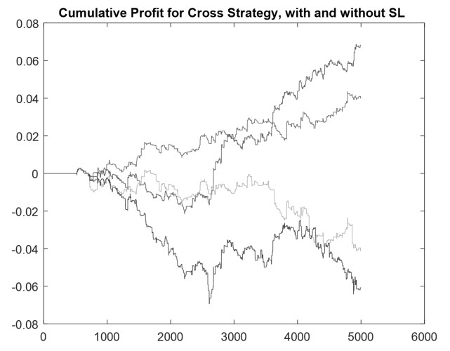
The article presents a certain investment strategy based on the difference between two moving averages, modified to allow the extraction of patterns. The strategy concept dropped the traditionally considered intersections of two averages and opening positions just after those intersections. Based on the observation of changes happening in the moving averages difference, it has been noticed that for some values of this difference and some values of additional strategy parameters, an interesting pattern appears that allows short-term prediction. These patterns also depended on the first derivative of the moving averages difference and the location of the current price relative to certain thresholds of the difference. Therefore, the strategy uses five parameters, including Stop Loss, adapted to the properties of the time series through machine learning. The importance of machine learning is highlighted by comparing simulation results with and without it. The strategy effectiveness was tested in the Matlab environment on the time series of the WIG20 (primary index of the Warsaw Stock Exchange) historical data. Satisfactory results were obtained considered in terms of minimizing investment risk measured by the Calmar indicator.
Citation: Antoni Wilinski, Mateusz Sochanowski, Wojciech Nowicki. An investment strategy based on the first derivative of the moving averages difference with parameters adapted by machine learning[J]. Data Science in Finance and Economics, 2022, 2(2): 96-116. doi: 10.3934/DSFE.2022005
The article presents a certain investment strategy based on the difference between two moving averages, modified to allow the extraction of patterns. The strategy concept dropped the traditionally considered intersections of two averages and opening positions just after those intersections. Based on the observation of changes happening in the moving averages difference, it has been noticed that for some values of this difference and some values of additional strategy parameters, an interesting pattern appears that allows short-term prediction. These patterns also depended on the first derivative of the moving averages difference and the location of the current price relative to certain thresholds of the difference. Therefore, the strategy uses five parameters, including Stop Loss, adapted to the properties of the time series through machine learning. The importance of machine learning is highlighted by comparing simulation results with and without it. The strategy effectiveness was tested in the Matlab environment on the time series of the WIG20 (primary index of the Warsaw Stock Exchange) historical data. Satisfactory results were obtained considered in terms of minimizing investment risk measured by the Calmar indicator.

| [1] |
Anderson BD, Deistler M, Felsenstein E, et al. (2016) The structure of multivariate AR and ARMA systems: Regular and singular systems; the single and the mixed frequency case. J Econometrics 192: 366–373. https://doi.org/10.1016/j.jeconom.2016.02.004 doi: 10.1016/j.jeconom.2016.02.004

|
| [2] |
Babu CN, Reddy BE (2014) A moving-average filter based hybrid ARIMA–ANN model for forecasting time series data. Appl Soft Comput 23: 27–38. https://doi.org/10.1016/j.asoc.2014.05.028 doi: 10.1016/j.asoc.2014.05.028
|
| [3] |
Brock W, Lakonishok J, LeBaron B (1992). Simple technical trading rules and the stochastic properties of stock returns. J Financ 47: 1731–1764. https://doi.org/10.1111/j.1540-6261.1992.tb04681.x doi: 10.1111/j.1540-6261.1992.tb04681.x
|
| [4] |
Chan JC (2013) Moving average stochastic volatility models with application to inflation forecast. J Econometrics 176: 162–172. https://doi.org/10.1016/j.jeconom.2013.05.003 doi: 10.1016/j.jeconom.2013.05.003
|
| [5] |
Dias GF, Kapetanios, G (2018) Estimation and forecasting in vector autoregressive moving average models for rich datasets. J Econometrics 202: 75–91. https://doi.org/10.1016/j.jeconom.2017.06.022 doi: 10.1016/j.jeconom.2017.06.022
|
| [6] |
Ellis CA, Parbery SA (2005) Is smarter better? A comparison of adaptive, and simple moving average trading strategies. Res Int Bus Financ 19: 399–411. https://doi.org/10.1016/j.ribaf.2004.12.009 doi: 10.1016/j.ribaf.2004.12.009
|
| [7] |
Gencay R (1998) The predictability of security returns with simple technical trading rules. J Empir Financ 5: 347–359. https://doi.org/10.1016/j.ribaf.2004.12.009 doi: 10.1016/j.ribaf.2004.12.009
|
| [8] |
Gencay R (1996). Non-linear prediction of security returns with moving average rules. J Forecasting 15: 165–174. https://doi.org/10.1002/(SICI)1099-131X(199604)15:3<165::AID-FOR617>3.0.CO;2-V doi: 10.1002/(SICI)1099-131X(199604)15:3<165::AID-FOR617>3.0.CO;2-V
|
| [9] | Hamilton JD (1994) Time series analysis. Princeton, NJ: Princeton university press. 2: 690–696 |
| [10] |
Horváth L, Rice G (2015) Testing for independence between functional time series. J Econometrics 189: 371–382. https://doi.org/10.1016/j.jeconom.2015.03.030 doi: 10.1016/j.jeconom.2015.03.030
|
| [11] | Johnston J, DiNardo J (1972) Econometric methods (Vol. 2). New York. |
| [12] | LeBaron B (1992) Do moving average trading rule results imply nonlinearities in foreign exchange markets? Social Systems Research Institute, University of Wisconsin. |
| [13] |
Ling S, McAleer M, Tong H (2015) Frontiers in time series and financial econometrics: An overview. J Econometrics 189: 145–250. https://doi.org/10.1016/j.jeconom.2015.03.019 doi: 10.1016/j.jeconom.2015.03.019
|
| [14] | Main R (2017) Evaluating Traders' Performers with the Calmar Ratio, www. proptradingfutures/thecalamr-ratio. Access J: www.proptradingfutures.com/the-calmar-ratio/. |
| [15] |
Metghalchi M, Marcucci J, Chang YH (2012) Are moving average trading rules profitable? Evidence from the European stock markets. Appl Econ 44: 1539–1559. https://doi.org/10.1080/00036846.2010.543084 doi: 10.1080/00036846.2010.543084
|
| [16] |
Moon YS, Kim J (2007) Efficient moving average transform-based subsequence matching algorithms in time-series databases. Inf Sci 177: 5415–5431. https://doi.org/10.1016/j.ins.2007.05.038 doi: 10.1016/j.ins.2007.05.038
|
| [17] | Murphy JJ (1999) Technical analysis of the financial markets: A comprehensive guide to trading methods and applications. Penguin. |
| [18] | Schwager JD (1984) A complete guide to the futures markets: fundamental analysis, technical analysis, trading, spreads, and options. John Wiley & Sons. |
| [19] | Schwager JD (1995) Technical analysis. (Vol. 43). John Wiley & Sons. |
| [20] | Wei WW (2006) Time series analysis. In The Oxford Handbook of Quantitative Methods in Psychology: Vol. 2. |
| [21] | Wilder JW (1978) New concepts in technical trading systems. Trend Research. |
| [22] | Yamane T (1973) Statistics: An introductory analysis. Researchgate.com |
| [23] | Young WT (1991) Calmar Ratio: A Smoother Tool. Futures 20: 40 |
| [24] |
Zhu K, Li WK (2015) A bootstrapped spectral test for adequacy in weak ARMA models. J Econometrics 187: 113–130. https://doi.org/10.1016/j.jeconom.2015.02.005 doi: 10.1016/j.jeconom.2015.02.005
|
| [25] |
Zhu Y, Zhou G (2009) Technical analysis: An asset allocation perspective on the use of moving averages. J Financ Econ 92: 519–544. https://doi.org/10.1016/j.jfineco.2008.07.002 doi: 10.1016/j.jfineco.2008.07.002
|
| [26] | Wilinski A (2011) Prediction Models of Financial Markets Based on Multiregression Algorithms, Comput Sci J Mold., vol. 19, no. 2, pp. 178–188, |
| [27] | Wilinski A, Zablocki M (2015) The Investment Strategy Based on the Difference of Moving Averages with Parameters Adapted by Machine Learning. Advanced in Intelligent Systems and Computing Springer, Cham Heidelberg New York, 342: 207–227 |


Figures(14) / Tables(1)
Antoni Wilinski, Mateusz Sochanowski, Wojciech Nowicki. An investment strategy based on the first derivative of the moving averages difference with parameters adapted by machine learning[J]. Data Science in Finance and Economics, 2022, 2(2): 96-116. doi: 10.3934/DSFE.2022005


 DownLoad: