Forecasting crude oil price using LSTM neural networks

Kexian Zhang; Min Hong; Kexian Zhang; Min Hong

doi:10.3934/DSFE.2022008

Data Science in Finance and Economics

2022, Volume 2, Issue 3: 163-180. doi: 10.3934/DSFE.2022008

Previous Article Next Article

Research article Special Issues

Forecasting crude oil price using LSTM neural networks

Kexian Zhang ^,,
Min Hong

School of Economics and Management, Hunan Institute of Technology, Hengyang 421002, China

Received: 20 February 2022 Revised: 09 May 2022 Accepted: 18 May 2022 Published: 07 July 2022
JEL Codes: C53, C81, C82, E37

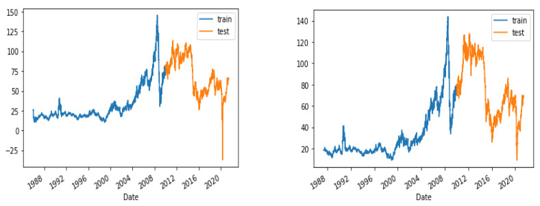
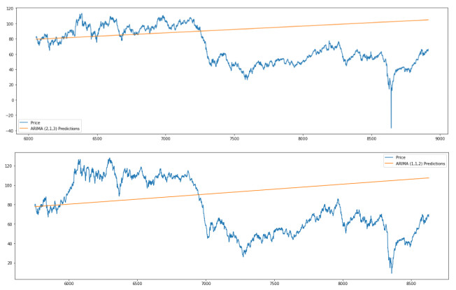
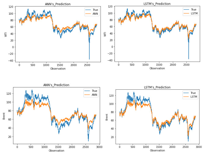
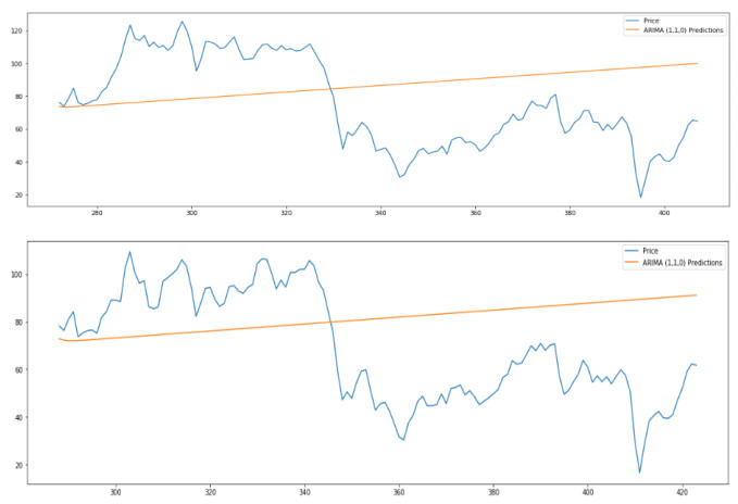
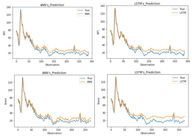
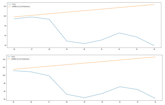
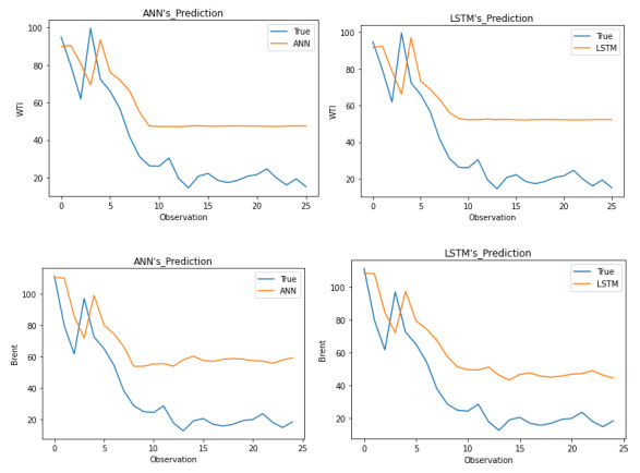
As a key input factor in industrial production, the price volatility of crude oil often brings about economic volatility, so forecasting crude oil price has always been a pivotal issue in economics. In our study, we constructed an LSTM (short for Long Short-Term Memory neural network) model to conduct this forecasting based on data from February 1986 to May 2021. An ANN (short for Artificial Neural Network) model and a typical ARIMA (short for Autoregressive Integrated Moving Average) model are taken as the comparable models. The results show that, first, the LSTM model has strong generalization ability, with stable applicability in forecasting crude oil prices with different timescales. Second, as compared to other models, the LSTM model generally has higher forecasting accuracy for crude oil prices with different timescales. Third, an LSTM model-derived shorter forecast price timescale corresponds to a lower forecasting accuracy. Therefore, given a longer forecast crude oil price timescale, other factors may need to be included in the model.
- crude oil price,
- forecast,
- LSTM neural network model,
- artificial neural networks,
- ARIMA
Citation: Kexian Zhang, Min Hong. Forecasting crude oil price using LSTM neural networks[J]. Data Science in Finance and Economics, 2022, 2(3): 163-180. doi: 10.3934/DSFE.2022008

Related Papers:

Abstract

As a key input factor in industrial production, the price volatility of crude oil often brings about economic volatility, so forecasting crude oil price has always been a pivotal issue in economics. In our study, we constructed an LSTM (short for Long Short-Term Memory neural network) model to conduct this forecasting based on data from February 1986 to May 2021. An ANN (short for Artificial Neural Network) model and a typical ARIMA (short for Autoregressive Integrated Moving Average) model are taken as the comparable models. The results show that, first, the LSTM model has strong generalization ability, with stable applicability in forecasting crude oil prices with different timescales. Second, as compared to other models, the LSTM model generally has higher forecasting accuracy for crude oil prices with different timescales. Third, an LSTM model-derived shorter forecast price timescale corresponds to a lower forecasting accuracy. Therefore, given a longer forecast crude oil price timescale, other factors may need to be included in the model.

References

[1]	Abdollahi H (2020) A Novel Hybrid Model for Forecasting Crude Oil Price Based on Time Series Decomposition. Appl Energy 267: 115035. https://doi.org/10.1016/j.apenergy.2020.115035 doi: 10.1016/j.apenergy.2020.115035
[2]	Aho K, Derryberry DW, Peterson T (2016) Model Selection for Ecologists: The Worldviews of Aic and Bic. Ecol 95: 631-636. https://www.jstor.org/stable/43495189
[3]	Ajmi AN, Hammoudeh S, Mokni K (2021) Detection of Bubbles in Wti, Brent, and Dubai Oil Prices: A Novel Double Recursive Algorithm. Resour Policy 70: 101956. https://doi.org/10.1016/j.resourpol.2020.101956 doi: 10.1016/j.resourpol.2020.101956
[4]	Azadeh A, Moghaddam M, Khakzad M, et al. (2012) A Flexible Neural Network-Fuzzy Mathematical Programming Algorithm for Improvement of Oil Price Estimation and Forecasting. Comput Indl Eng 62: 421-30. https://doi.org/10.1016/j.cie.2011.06.019 doi: 10.1016/j.cie.2011.06.019
[5]	Butler S, Kokoszka P, Miao H, et al. (2021) Neural Network Prediction of Crude Oil Futures Using B-Splines. Energy Econ 94: 105080. https://doi.org/10.1016/j.eneco.2020.105080 doi: 10.1016/j.eneco.2020.105080
[6]	Chen L, Zhang Z, Chen F, et al. (2019) A Study on the Relationship between Economic Growth and Energy Consumption under the New Normal. Natl Account Rev 1: 28-41. https://doi.org/10.3934/nar.2019.1.28 doi: 10.3934/NAR.2019.1.28
[7]	Chiroma H, Abdulkareem S, Herawan T (2015) Evolutionary Neural Network Model for West Texas Intermediate Crude Oil Price Prediction. Appl Energy 142: 266-273. https://doi.org/10.1016/j.apenergy.2014.12.045 doi: 10.1016/j.apenergy.2014.12.045
[8]	Fan D, Sun H, Yao J, et al. (2021) Well Production Forecasting Based on Arima-Lstm Model Considering Manual Operations. Energy 220: 119708. https://doi.org/10.1016/j.energy.2020.119708 doi: 10.1016/j.energy.2020.119708
[9]	Fischer T, Krauss C (2018) Deep Learning with Long Short-Term Memory Networks for Financial Market Predictions. Eur J Oper Res 270: 654-669. https://doi.org/10.1016/j.ejor.2017.11.054 doi: 10.1016/j.ejor.2017.11.054
[10]	Gori F, Ludovisi D, Cerritelli P (2007) Forecast of Oil Price and Consumption in the Short Term under Three Scenarios: Parabolic, Linear and Chaotic Behaviour. Energy 32: 1291-1296. https://doi.org/10.1016/j.energy.2006.07.005 doi: 10.1016/j.energy.2006.07.005
[11]	Grace SP, Kanamura T (2020) Examining Risk and Return Profiles of Renewable Energy Investment in Developing Countries: The Case of the Philippines. Green Financ 2: 135-150. https://doi.org/10.3934/gf.2020008 doi: 10.3934/GF.2020008
[12]	Graves A (2012) Long Short-Term Memory, A. Graves, Supervised Sequence Labelling with Recurrent Neural Networks. Berlin, Heidelberg: Springer Berlin Heidelberg, 37-45.
[13]	He K, Yu L, Lai KK (2012) Crude Oil Price Analysis and Forecasting Using Wavelet Decomposed Ensemble Model. Energy 46: 564-574. https://doi.org/10.1016/j.energy.2012.07.055 doi: 10.1016/j.energy.2012.07.055
[14]	Hochreiter S, Schmidhuber J (1997) Long Short-Term Memory. Neural comput 9: 1735-1780. https://doi.org/10.1162/neco.1997.9.8.1735 doi: 10.1162/neco.1997.9.8.1735
[15]	James DH (2009) Causes and Consequences of the Oil Shock of 2007-08. Brookings Papers on Economic Activity 215-261. https://doi.org/10.1353/eca.0.0047 doi: 10.1353/eca.0.0047
[16]	Lammerding M, Stephan P, Trede M, et al. (2013) Speculative Bubbles in Recent Oil Price Dynamics: Evidence from a Bayesian Markov-Switching State-Space Approach. Energy Econ 36: 491-502. https://doi.org/10.1016/j.eneco.2012.10.006 doi: 10.1016/j.eneco.2012.10.006
[17]	Li T, Liao G (2020) The Heterogeneous Impact of Financial Development on Green Total Factor Productivity. Front Energy Res 8: 29. https://doi.org/10.3389/fenrg.2020.00029 doi: 10.3389/fenrg.2020.00029
[18]	Li T, Zhong J, Huang Z (2020a) Potential Dependence of Financial Cycles between Emerging and Developed Countries: Based on Arima-Garch Copula Model. Emerg Mark Financ Trade 56: 1237-1250. https://doi.org/10.1080/1540496X.2019.1611559 doi: 10.1080/1540496X.2019.1611559
[19]	Li X, Shang W, Wang S (2019) Text-Based Crude Oil Price Forecasting: A Deep Learning Approach. Int J Forecasting 35: 1548-60. https://doi.org/10.1016/j.ijforecast.2018.07.006 doi: 10.1016/j.ijforecast.2018.07.006
[20]	Li Z, Dong H, Floros C, et al. (2021) Re-Examining Bitcoin Volatility: A Caviar-Based Approach. Emerg Mark Financ Trade: 1-19. https://doi.org/10.1080/1540496X.2021.1873127 doi: 10.1080/1540496X.2021.1873127
[21]	Li Z, Wang Y, Huang Z (2020b) Risk Connectedness Heterogeneity in the Cryptocurrency Markets. Front Phys 8: 243. https://doi.org/10.3389/fphy.2020.00243 doi: 10.3389/fphy.2020.00243
[22]	Lin Y, Xiao Y, Li F (2020) Forecasting Crude Oil Price Volatility Via a Hm-Egarch Model. Energy Econ 87: 104693. https://doi.org/10.1016/j.eneco.2020.104693 doi: 10.1016/j.eneco.2020.104693
[23]	Lu Q, Li Y, Chai J, et al. (2020) Crude Oil Price Analysis and Forecasting: A Perspective of "New Triangle". Energy Econs 87: 104721. https://doi.org/10.1016/j.eneco.2020.104721 doi: 10.1016/j.eneco.2020.104721
[24]	Mostafa MM, El-Masry AA (2016) Oil Price Forecasting Using Gene Expression Programming and Artificial Neural Networks. Econ Model 54: 40-53. https://doi.org/10.1016/j.econmod.2015.12.014 doi: 10.1016/j.econmod.2015.12.014
[25]	Murat A, Tokat E (2009) Forecasting Oil Price Movements with Crack Spread Futures. Energy Econ 31: 85-90. https://doi.org/10.1016/j.eneco.2008.07.008 doi: 10.1016/j.eneco.2008.07.008
[26]	Nonejad N (2020) Should Crude Oil Price Volatility Receive More Attention Than the Price of Crude Oil? An Empirical Investigation Via a Large-Scale out-of-Sample Forecast Evaluation of Us Macroeconomic Data. J Forecasting. https://doi.org/10.1002/for.2738 doi: 10.1002/for.2738
[27]	Ouyang ZS, Yang XT, Lai Y (2021) Systemic Financial Risk Early Warning of Financial Market in China Using Attention-Lstm Model. North Am J Econ Financ 56: 101383. https://doi.org/10.1016/j.najef.2021.101383 doi: 10.1016/j.najef.2021.101383
[28]	Pabuçcu H, Ongan S, Ongan A (2020) Forecasting the Movements of Bitcoin Prices: An Application of Machine Learning Algorithms. Quant Financ Econ 4: 679-692. https://doi.org/10.3934/qfe.2020031 doi: 10.3934/QFE.2020031
[29]	Ramyar S, Kianfar F (2017) Forecasting Crude Oil Prices: A Comparison between Artificial Neural Networks and Vector Autoregressive Models. Comput Econ 53: 743-761. https://doi.org/10.1007/s10614-017-9764-7 doi: 10.1007/s10614-017-9764-7
[30]	Shibata R (1976) Selection of the Order of an Autoregressive Model by Akaike's Information Criterion. Biometrika 63: 117-126. https://doi.org/10.1093/biomet/63.1.117 doi: 10.1093/biomet/63.1.117
[31]	Wei Y, Wang Y, Huang D (2010) Forecasting Crude Oil Market Volatility: Further Evidence Using Garch-Class Models. Energy Econ 32: 1477-1484. https://doi.org/10.1016/j.eneco.2010.07.009 doi: 10.1016/j.eneco.2010.07.009
[32]	Yu L, Dai W, Tang L, et al. (2015) A Hybrid Grid-Ga-Based Lssvr Learning Paradigm for Crude Oil Price Forecasting. Neural Comput Appls 27: 2193-2215. https://doi.org/10.1007/s00521-015-1999-4 doi: 10.1007/s00521-015-1999-4
[33]	Yu L, Zha R, Stafylas D, et al. (2020) Dependences and Volatility Spillovers between the Oil and Stock Markets: New Evidence from the Copula and Var-Bekk-Garch Models. Int Rev Financ Anal 68. https://doi.org/10.1016/j.irfa.2018.11.007 doi: 10.1016/j.irfa.2018.11.007
[34]	Zhang JL, Zhang YJ, Zhang L (2015) A Novel Hybrid Method for Crude Oil Price Forecasting. Energy Econ 49: 649-659. https://doi.org/10.1016/j.eneco.2015.02.018 doi: 10.1016/j.eneco.2015.02.018
[35]	Zhang Y, Ma F, Wang Y (2019) Forecasting Crude Oil Prices with a Large Set of Predictors: Can Lasso Select Powerful Predictors? J Empir Financ 54: 97-117. https://doi.org/10.1016/j.jempfin.2019.08.007 doi: 10.1016/j.jempfin.2019.08.007
[36]	Zhao Y, Li J, Yu L (2017) A Deep Learning Ensemble Approach for Crude Oil Price Forecasting. Energy Econ 66: 9-16. https://doi.org/10.1016/j.eneco.2017.05.023 doi: 10.1016/j.eneco.2017.05.023
[37]	Zheng Y, Du Z (2019) A Systematic Review in Crude Oil Markets: Embarking on the Oil Price. Green Financ 1: 328-345. https://doi.org/10.3934/gf.2019.3.328 doi: 10.3934/GF.2019.3.328
[38]	Zhong J, Wang M, M Drakeford B, et al. (2019) Spillover Effects between Oil and Natural Gas Prices: Evidence from Emerging and Developed Markets. Green Financ 1: 30-45. https://doi.org/10.3934/gf.2019.1.30 doi: 10.3934/GF.2019.1.30

Reader Comments

Your name:*

Email:*
© 2022 the Author(s), licensee AIMS Press. This is an open access article distributed under the terms of the Creative Commons Attribution License (http://creativecommons.org/licenses/by/4.0)