This paper investigates the impact of oil market structural shocks on the prices of natural gas liquids (NGLs), including ethane, propane, normal butane, isobutane, and natural gasoline, over the period from January 1985 to April 2020. To identify the structural demand and supply shocks in the crude oil market, we use a vector autoregression model and assume that the innovations to the real price of crude oil are predetermined with respect to the local NGLs markets. Our results show that, in the long run, more than 55% of the variation in the real price of NGLs is explained by the structural shocks in the global crude oil market. We also find that, unlike oil supply shocks, demand-side shocks have permanent and persistent impacts on NGLs' real prices and should be of main concern to investors aiming to develop gas wells and NGLs producing technologies.
Citation: Ali Jadidzadeh, Apostolos Serletis. Oil prices and the natural gas liquids markets[J]. Green Finance, 2022, 4(2): 207-230. doi: 10.3934/GF.2022010
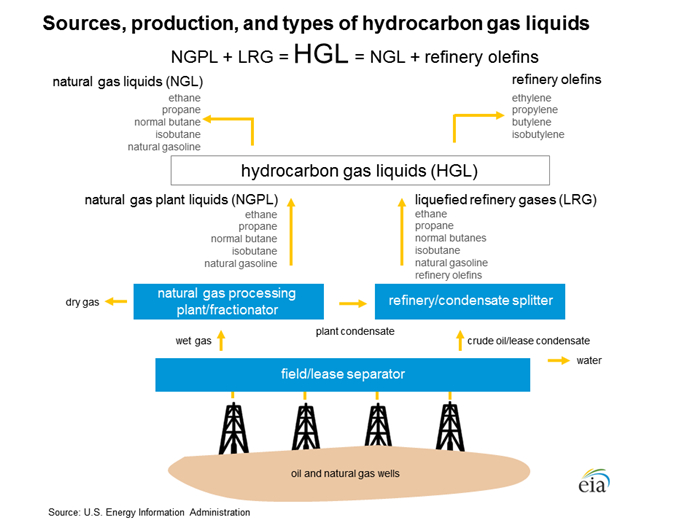
This paper investigates the impact of oil market structural shocks on the prices of natural gas liquids (NGLs), including ethane, propane, normal butane, isobutane, and natural gasoline, over the period from January 1985 to April 2020. To identify the structural demand and supply shocks in the crude oil market, we use a vector autoregression model and assume that the innovations to the real price of crude oil are predetermined with respect to the local NGLs markets. Our results show that, in the long run, more than 55% of the variation in the real price of NGLs is explained by the structural shocks in the global crude oil market. We also find that, unlike oil supply shocks, demand-side shocks have permanent and persistent impacts on NGLs' real prices and should be of main concern to investors aiming to develop gas wells and NGLs producing technologies.

| [1] |
Alquist R, Kilian L (2010) What do we learn from the price of crude oil futures? J Appl Econometrics 25: 539–573. https://doi.org/10.1002/jae.1159 doi: 10.1002/jae.1159

|
| [2] | Boersma T, Ebinger CK, Greenley HL (2015) An assessment of U.S. natural gas exports. The Brookings Institution, Washington, DC., 1–22. |
| [3] |
Diaz EM, de Gracia FP (2017) Oil price shocks and stock returns of oil and gas corporations. Financ Res Lett 20: 75–80. https://doi.org/10.1016/j.frl.2016.09.010 doi: 10.1016/j.frl.2016.09.010
|
| [4] | Energy Information Administration (2014) Hydrocarbon Gas Liquids (HGL): Recent market trends and issues. U.S. Energy Information Administration, U.S. Department of Energy, Washington, DC. Available from: eia.gov/analysis/hgl/pdf/hgl.pdf. |
| [5] |
Gonçalves S, Kilian L (2004) Bootstrapping autoregressions with conditional heteroskedasticity of unknown form. J Econometrics 123: 89–120. https://doi.org/10.1016/j.jeconom.2003.10.030 doi: 10.1016/j.jeconom.2003.10.030
|
| [6] |
Jadidzadeh A, Serletis A (2017) How does the US natural gas market react to demand and supply shocks in the crude oil market? Energy Econ 63: 66–74. https://doi.org/10.1016/j.eneco.2017.01.007 doi: 10.1016/j.eneco.2017.01.007
|
| [7] |
Kang W, de Gracia FP, Ratti RA (2017) Oil price shocks, policy uncertainty, and stock returns of oil and gas corporations. J Int Money Financ 70: 344–359. https://doi.org/10.1016/j.jimonfin.2016.10.003 doi: 10.1016/j.jimonfin.2016.10.003
|
| [8] |
Kassouri Y, Altıntaş H (2021) The quantile dependence of the stock returns of "clean" and "dirty" firms on oil demand and supply shocks. J Commod Mark, 100238. https://doi.org/10.1016/j.jcomm.2021.100238 doi: 10.1016/j.jcomm.2021.100238
|
| [9] |
Kassouri Y, Bilgili F, Kuşkaya S (2022) A wavelet-based model of world oil shocks interaction with CO$_2$ emissions in the US. Environ Sci & Policy 127: 280–292. https://doi.org/10.1016/j.envsci.2021.10.020 doi: 10.1016/j.envsci.2021.10.020
|
| [10] |
Kilian L (2009) Not all oil price shocks are alike: Disentangling demand and supply shocks in the crude oil market. Am Econ Rev 99: 1053–1069. https://doi.org/10.1257/aer.99.3.1053 doi: 10.1257/aer.99.3.1053
|
| [11] |
Kilian L (2010) Explaining fluctuations in gasoline prices: A joint model of the global crude oil market and the U.S. retail gasoline market. Energy J 99: 87–112. https://doi.org/10.5547/ISSN0195-6574-EJ-Vol31-No2-4 doi: 10.5547/ISSN0195-6574-EJ-Vol31-No2-4
|
| [12] |
Kilian L, Murphy DP (2014) The role of inventories and speculative trading in the global market for crude oil. J AppL Econometrics 29: 454–478. https://doi.org/10.1002/jae.2322 doi: 10.1002/jae.2322
|
| [13] |
Kilian L, Park C (2009) The impact of oil price shocks on the us stock market. Int Econ Rev 50: 1267–1287. https://doi.org/10.1111/j.1468-2354.2009.00568.x doi: 10.1111/j.1468-2354.2009.00568.x
|
| [14] | Light M (2014) Natural gas based liquid fuels: potential investment opportunities in the United States. University of Colorado Boulder, 1–18. |
| [15] |
Lütkepohl H, Netšunajev A (2014) Disentangling demand and supply shocks in the crude oil market: How to check sign restrictions in structural VARs. J Appl Econometrics 29: 479–496. https://doi.org/10.1002/jae.2330 doi: 10.1002/jae.2330
|
| [16] |
Oglend A, Lindbäck ME, Osmundsen P (2015) Shale gas boom affecting the relationship between LPG and oil prices. Energy J 36: 265–286. https://doi.org/10.5547/01956574.36.4.aogl doi: 10.5547/01956574.36.4.aogl
|
| [17] |
Rui X, Feng L, Feng J (2020) A gas-on-gas competition trading mechanism based on cooperative game models in China's gas market. Energy Rep 6: 365–377. https://doi.org/10.1016/j.egyr.2020.01.015 doi: 10.1016/j.egyr.2020.01.015
|
| [18] | Wamsley RK (2000) Natural gas liquid allocations. Petroleum Accounting Financ Manage J 19: 1–16. |


Figures(13) / Tables(7)

Ali Jadidzadeh, Apostolos Serletis. Oil prices and the natural gas liquids markets[J]. Green Finance, 2022, 4(2): 207-230. doi: 10.3934/GF.2022010


 DownLoad: