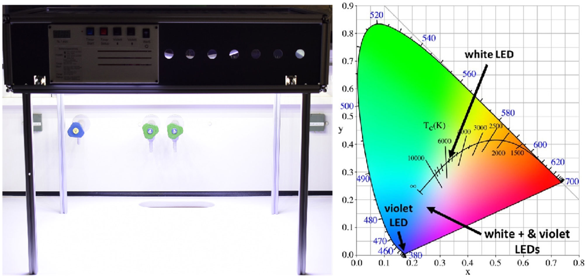
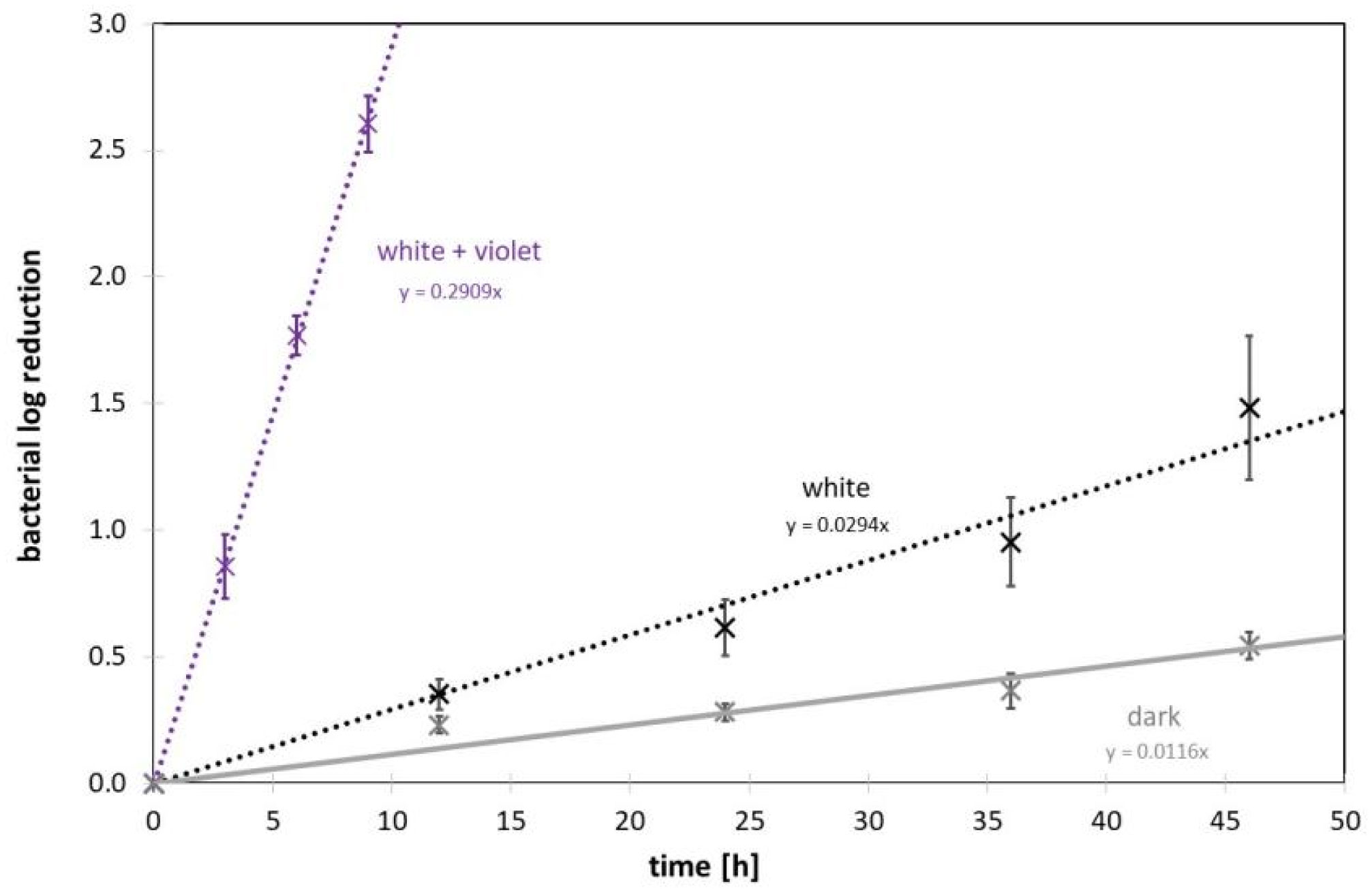
The spread of infections, as in the coronavirus pandemic, leads to the desire to perform disinfection measures even in the presence of humans. UVC radiation is known for its strong antimicrobial effect, but it is also harmful to humans. Visible light, on the other hand, does not affect humans and laboratory experiments have already demonstrated that intense visible violet and blue light has a reducing effect on bacteria and viruses. This raises the question of whether the development of pathogen-reducing illumination is feasible for everyday applications. For this purpose, a lighting device with white and violet LEDs is set up to illuminate a work surface with 2,400 lux of white light and additionally with up to 2.5 mW/cm2 of violet light (405 nm). Staphylococci are evenly distributed on the work surface and the decrease in staphylococci concentration is observed over a period of 46 hours. In fact, the staphylococci concentration decreases, but with the white illumination, a 90% reduction occurs only after 34 hours; with the additional violet illumination the necessary irradiation time is shortened to approx. 3.5 hours. Increasing the violet component probably increases the disinfection effect, but the color impression moves further away from white and the low disinfection durations of UVC radiation can nevertheless not be achieved, even with very high violet emissions.
Citation: Martin Hessling, Tobias Meurle, Katharina Hoenes. Surface disinfection with white-violet illumination device[J]. AIMS Bioengineering, 2022, 9(2): 93-101. doi: 10.3934/bioeng.2022008
The spread of infections, as in the coronavirus pandemic, leads to the desire to perform disinfection measures even in the presence of humans. UVC radiation is known for its strong antimicrobial effect, but it is also harmful to humans. Visible light, on the other hand, does not affect humans and laboratory experiments have already demonstrated that intense visible violet and blue light has a reducing effect on bacteria and viruses. This raises the question of whether the development of pathogen-reducing illumination is feasible for everyday applications. For this purpose, a lighting device with white and violet LEDs is set up to illuminate a work surface with 2,400 lux of white light and additionally with up to 2.5 mW/cm2 of violet light (405 nm). Staphylococci are evenly distributed on the work surface and the decrease in staphylococci concentration is observed over a period of 46 hours. In fact, the staphylococci concentration decreases, but with the white illumination, a 90% reduction occurs only after 34 hours; with the additional violet illumination the necessary irradiation time is shortened to approx. 3.5 hours. Increasing the violet component probably increases the disinfection effect, but the color impression moves further away from white and the low disinfection durations of UVC radiation can nevertheless not be achieved, even with very high violet emissions.

| [1] | Coronavirus Resource Center, COVID-19 Dashboard: (Global Map), 2022. Available from: https://coronavirus.jhu.edu/map.html |
| [2] |
Murray CJL, Ikuta KS, Sharara F, et al. (2022) Global burden of bacterial antimicrobial resistance in 2019: a systematic analysis. The Lancet 399: 629-655. https://doi.org/10.1016/S0140-6736(21)02724-0 
|
| [3] |
Jagger J (1968) Introduction to research in ultraviolet photobiology. Photochem Photobiol 7: 413.
|
| [4] |
Masjoudi M, Mohseni M, Bolton JR (2021) Sensitivity of bacteria, protozoa, viruses, and other microorganisms to ultraviolet radiation. J Res Natl Inst Stan 126: 1-77. https://doi.org/10.6028/jres.126.021
|
| [5] |
Kowalski W (2009) Ultraviolet Germicidal Irradiation Handbook. Berlin: Springer.
|
| [6] |
Liu S, Luo W, Li D, et al. (2021) Sec-eliminating the SARS-CoV-2 by AlGaN based high power deep ultraviolet light source. Adv Funct Mater 31: 2008452. https://doi.org/10.1002/adfm.202008452
|
| [7] |
Rathnasinghe R, Karlicek RF, Schotsaert M, et al. (2021) Scalable, effective, and rapid decontamination of SARS-CoV-2 contaminated N95 respirators using germicidal ultraviolet C (UVC) irradiation device. Sci Rep 11: 1-10. https://doi.org/10.1038/s41598-021-99431-5
|
| [8] |
Ruetalo N, Businger R, Schindler M (2021) Rapid, dose-dependent and efficient inactivation of surface dried SARS-CoV-2 by 254 nm UV-C irradiation. Eurosurveillance 26: 2001718. https://doi.org/10.2807/1560-7917.ES.2021.26.42.2001718
|
| [9] |
Ashkenazi H, Malik Z, Harth Y, et al. (2003) Eradication of Propionibacterium acnes by its endogenic porphyrins after illumination with high intensity blue light. FEMS Immunol Med Microbiol 35: 17-24. https://doi.org/10.1111/j.1574-695X.2003.tb00644.x
|
| [10] |
Guffey JS, Wilborn J (2006) In vitro bactericidal effects of 405-nm and 470-nm blue light. Photomed Laser Ther 24: 684-688. https://doi.org/10.1089/pho.2006.24.684
|
| [11] |
Maclean M, MacGregor SJ, Anderson JG, et al. (2008) High-intensity narrow-spectrum light inactivation and wavelength sensitivity of Staphylococcus aureus. FEM Microbiol Lett 285: 227-232. https://doi.org/10.1111/j.1574-6968.2008.01233.x
|
| [12] |
Feuerstein O, Ginsburg I, Dayan E, et al. (2005) Mechanism of visible light phototoxicity on Porphyromonas gingivalis and Fusobacterium nucleatum. Photochem Photobiol 81: 1186-1189. https://doi.org/10.1562/2005-04-06-RA-477
|
| [13] |
Amin RM, Bhayana B, Hamblin MR, et al. (2016) Antimicrobial blue light inactivation of Pseudomonas aeruginosa by photo-excitation of endogenous porphyrins: in vitro and in vivo studies. Laser Surg Med 48: 562-568. https://doi.org/10.1002/lsm.22474
|
| [14] |
Plavskii VY, Mikulich AV, Tretyakova AI, et al. (2018) Porphyrins and flavins as endogenous acceptors of optical radiation of blue spectral region determining photoinactivation of microbial cells. J Photochem Photobiol B 183: 172-183. https://doi.org/10.1016/j.jphotobiol.2018.04.021
|
| [15] |
Cieplik F, Späth A, Leibl C, et al. (2014) Blue light kills aggregatibacter actinomycetemcomitans due to its endogenous photosensitizers. Clin Oral Invest 18: 1763-1769. https://doi.org/10.1007/s00784-013-1151-8
|
| [16] |
Hessling M, Spellerberg B, Hoenes K (2017) Photoinactivation of bacteria by endogenous photosensitizers and exposure to visible light of different wavelengths–a review on existing data. FEM Microbiol Lett 364: fnw270. https://doi.org/10.1093/femsle/fnw270
|
| [17] |
Tomb RM, White TA, Coia JE, et al. (2018) Review of the comparative susceptibility of microbial species to photoinactivation using 380–480 nm violet-blue light. Photochem Photobiol 94: 445-458. https://doi.org/10.1111/php.12883
|
| [18] |
Hessling M, Lau B, Vatter P (2022) Review of virus inactivation by visible light. Photonics 9: 113. https://doi.org/10.3390/photonics9020113
|
| [19] |
Kleinpenning MM, Smits T, Frunt MHA, et al. (2010) Clinical and histological effects of blue light on normal skin. Photodermatol Photoimmunol Photome 26: 16-21. https://doi.org/10.1111/j.1600-0781.2009.00474.x
|
| [20] |
McDonald R, Gupta S, MacLean M, et al. (2013) 405 nm light exposure of osteoblasts and inactivation of bacterial isolates from arthroplasty patients: potential for new disinfection applications?. Eur Cells Mater 25: 204-214. https://doi.org/10.22203/eCM.v025a15
|
| [21] |
Gillespie JB, Maclean M, Wilson MP, et al. (2017) Development of an antimicrobial blended white LED system containing pulsed 405nm LEDs for decontamination applications. Proc SPIE 10056: 100560Y. https://doi.org/10.1117/12.2250539
|
| [22] |
Rohan A, Khan I, Yin D, et al. (2019) Passive ceiling light disinfection system to reduce bioburden in an intensive care unit. J Pediatr Intensive 8: 138-143. https://doi.org/10.1055/s-0038-1676655
|
| [23] |
Rutala WA, Kanamori H, Gergen MF, et al. (2018) Antimicrobial activity of a continuous visible light disinfection system. Infect Control Hosp Epidemiol 39: 1250-1253. https://doi.org/10.1017/ice.2018.200
|
| [24] |
Buehler J, Sommerfeld F, Meurle T, et al. (2021) Disinfection properties of conventional white LED illumination and their potential increase by violet LEDs for applications in medical and domestic environments. Adv Sci Technol Res J 15: 169-175. https://doi.org/10.12913/22998624/134641
|
| [25] |
Hoenes K, Bauer R, Meurle T, et al. (2021) Inactivation effect of violet and blue light on ESKAPE pathogens and closely related non-pathogenic bacterial species–a promising tool against antibiotic-sensitive and antibiotic-resistant microorganisms. Front Microbiol 11: 612367. https://doi.org/10.3389/fmicb.2020.612367
|
| [26] |
Lau B, Becher D, Hessling M (2021) High intensity violet light (405 nm) inactivates coronaviruses in phosphate buffered saline (PBS) and on surfaces. Photonics 8: 414. https://doi.org/10.3390/photonics8100414
|
| [27] | Amerlux LLC, Active Clean: Nonstop Antimicrobial Action Against Viruses and Bacteria, 2021. Available from: https://bestlight.amerlux.com/active-clean/ |
| [28] | User Par, Planckian Locus, 2012. Available from: https://commons.wikimedia.org/wiki/File:PlanckianLocus.png |
| [29] | DIN EN 12464-1:2021-11, Light and lighting-Lighting of work places-Part 1: Indoor work places, Beuth Verlag GmbH, Berlin. Available from: https://standards.globalspec.com/std/14462596/EN%2012464-1 |
| [30] |
Michelini Z, Mazzei C, Magurano F, et al. (2021) UltraViolet SANitizing system for sterilization of ambulances fleets and for real-time monitoring of their sterilization level. Int J Environ Res Public Health 19: 331. https://doi.org/10.3390/ijerph19010331
|
| [31] |
Yang JH, Wu UI, Tai HM, et al. (2019) Effectiveness of an ultraviolet-C disinfection system for reduction of healthcare-associated pathogens. J Microbiol Immunol Infect 52: 487-493. https://doi.org/10.1016/j.jmii.2017.08.017
|
| [32] |
Rutala WA, Gergen MF, Tande BM, et al. (2013) Rapid hospital room decontamination using ultraviolet (UV) light with a nanostructured UV-reflective wall coating. Infect Control Hosp Epidemiol 34: 527-529. https://doi.org/10.1086/670211
|
| [33] |
Bormann M, Alt M, Schipper L, et al. (2021) Disinfection of SARS-CoV-2 contaminated surfaces of personal items with UVC-LED disinfection boxes. Viruses 13: 598. https://doi.org/10.3390/v13040598
|
| [34] |
Rutala WA, Gergen MF, Tande BM, et al. (2014) Room decontamination using an ultraviolet-C device with short ultraviolet exposure time. Infect Control Hosp Epidemiol 35: 1070-1072. https://doi.org/10.1086/677149
|
| [35] |
Rutala WA, Gergen MF, Weber DJ (2010) Room decontamination with UV radiation. Infect Control Hosp Epidemiol 31: 1025-1029. https://doi.org/10.1086/656244
|
| [36] |
McDevitt JJ, Milton DK, Rudnick SN, et al. (2008) Inactivation of poxviruses by upper-room UVC light in a simulated hospital room environment. PLoS One 3: e3186. https://doi.org/10.1371/journal.pone.0003186
|
| [37] |
Bedell K, Buchaklian AH, Perlman S (2016) Efficacy of an automated multiple emitter whole-room ultraviolet-C disinfection system against coronaviruses MHV and MERS-CoV. Infect Control Hosp Epidemiol 37: 598-599. https://doi.org/10.1017/ice.2015.348
|
| [38] |
Nunayon SS, Zhang H, Lai ACK (2020) Comparison of disinfection performance of UVC-LED and conventional upper-room UVGI systems. Indoor Air 30: 180-191. https://doi.org/10.1111/ina.12619
|
| [39] |
Szeto W, Yam WC, Huang H, et al. (2020) The efficacy of vacuum-ultraviolet light disinfection of some common environmental pathogens. BMC Infect Dis 20: 1-9. https://doi.org/10.1186/s12879-020-4847-9
|
Figures(2)

Martin Hessling, Tobias Meurle, Katharina Hoenes. Surface disinfection with white-violet illumination device[J]. AIMS Bioengineering, 2022, 9(2): 93-101. doi: 10.3934/bioeng.2022008


 DownLoad: