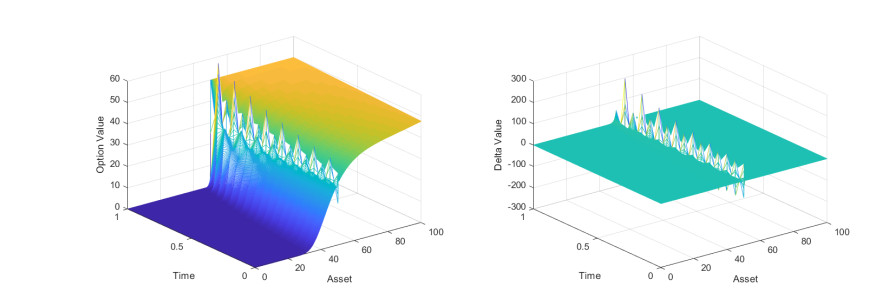
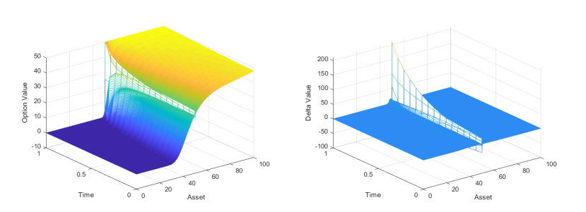
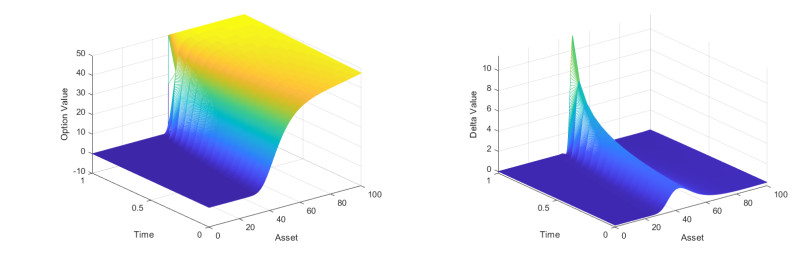
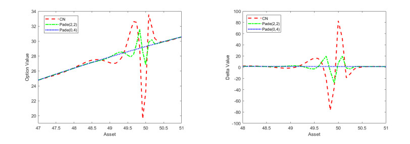
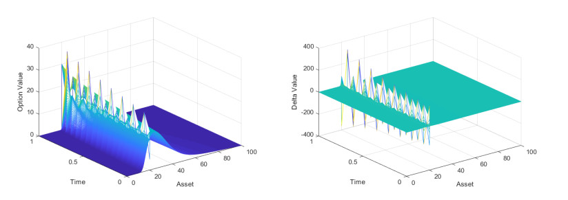
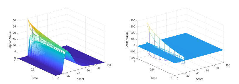
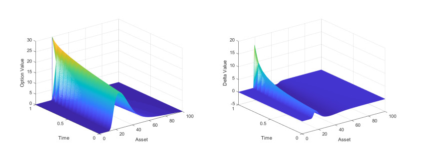
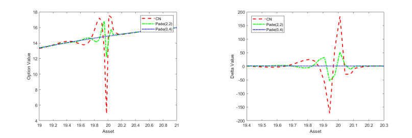
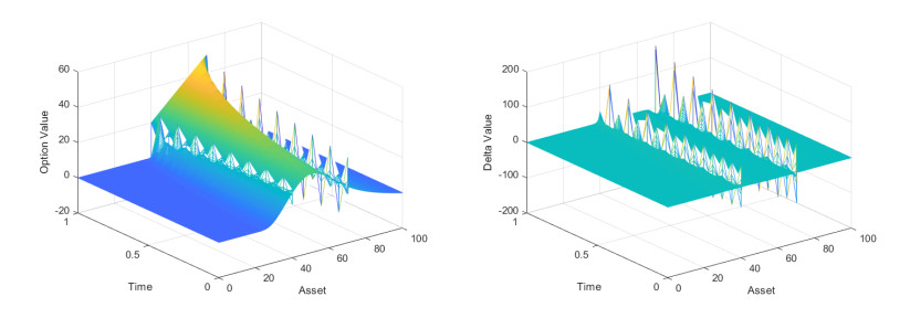
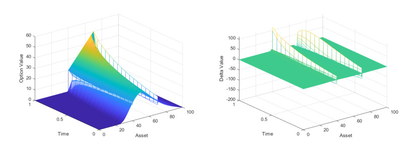
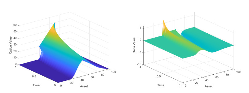
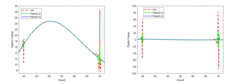
In order to reduce the oscillations of the numerical solution of fractional exotic options pricing model, a class of numerical schemes are developed and well studied in this paper which are based on the 4th-order Padé approximation and 2nd-order weighted and shifted Grünwald difference scheme. Since the spatial discretization matrix is positive definite and has lower Hessenberg Toeplitz structure, we prove the convergence of the proposed scheme. Numerical experiments on fractional digital option and fractional barrier options show that the (0, 4)-Padé scheme is fast, and significantly reduces the oscillations of the solution and smooths the Delta value.
Citation: Ming-Kai Wang, Cheng Wang, Jun-Feng Yin. A class of fourth-order Padé schemes for fractional exotic options pricing model[J]. Electronic Research Archive, 2022, 30(3): 874-897. doi: 10.3934/era.2022046
In order to reduce the oscillations of the numerical solution of fractional exotic options pricing model, a class of numerical schemes are developed and well studied in this paper which are based on the 4th-order Padé approximation and 2nd-order weighted and shifted Grünwald difference scheme. Since the spatial discretization matrix is positive definite and has lower Hessenberg Toeplitz structure, we prove the convergence of the proposed scheme. Numerical experiments on fractional digital option and fractional barrier options show that the (0, 4)-Padé scheme is fast, and significantly reduces the oscillations of the solution and smooths the Delta value.

| [1] |
F. Black, M. Scholes, The pricing of options and corporate liabilities, J. Political Economy, 81 (1973), 637–654. https://doi.org/10.1086/260062 doi: 10.1086/260062

|
| [2] |
R. C. Merton, Theory of rational option pricing, Bell J. Econ. Manage. Sci., 4 (1973), 141–183. https://doi.org/10.2307/3003143 doi: 10.2307/3003143
|
| [3] |
R. C. Merton, Option pricing when underlying stock returns are discontinuous, J. Financ. Econ., 3 (1976), 125–144. https://doi.org/10.1016/0304-405X(76)90022-2 doi: 10.1016/0304-405X(76)90022-2
|
| [4] | S. Heston, A closed-form solution for options with stochastic volatility with applications to bond and currency options, Review of Financ. Stud., 6 (1993), 327–343. Available from: https://www.jstor.org/stable/2962057. |
| [5] |
A. White, J. Hull, The pricing of options on assets with stochastic volatilities, J. Finance, 42 (1987), 281–300. https://doi.org/10.1111/j.1540-6261.1987.tb02568.x doi: 10.1111/j.1540-6261.1987.tb02568.x
|
| [6] |
P. Carr, L. Wu, The finite moment log stable process and option pricing, J. Finance, 58 (2003), 753–777. https://doi.org/10.1111/1540-6261.00544 doi: 10.1111/1540-6261.00544
|
| [7] |
I. Koponen, Analytic approach to the problem of convergence of truncated Lévy flights towards the Gaussian stochastic process, Phys. Rev. E, 52 (1995), 1197. https://doi.org/10.1103/PhysRevE.52.1197 doi: 10.1103/PhysRevE.52.1197
|
| [8] |
L. X. Zhang, R. F. Peng, J. F. Yin, A second order numerical scheme for fractional option pricing models, East Asian J. Appl. Math., 11 (2021), 326–348. https://doi.org/10.4208/eajam.020820.121120 doi: 10.4208/eajam.020820.121120
|
| [9] |
P. Carr, H. Geman, D. B. Madan, M. Yor, Stochastic volatility for Lévy processes, Math. Finance, 13 (2003), 345–382. https://doi.org/10.1111/1467-9965.00020 doi: 10.1111/1467-9965.00020
|
| [10] | R. Cont, E. Voltchkova, A finite difference scheme for option pricing in jump diffusion and exponential lévy models, SIAM J. Numer. Anal., 43 (2005), 1596–1626. https://doi.org/10.1137/S0036142903436186 |
| [11] |
Á. Cartea, D. del Castillo-Negrete, Fractional diffusion models of option prices in markets with jumps, Physica A, 374 (2007), 749–763. https://doi.org/10.1016/j.physa.2006.08.071 doi: 10.1016/j.physa.2006.08.071
|
| [12] |
O. Marom, E. Momoniat, A comparison of numerical solutions of fractional diffusion models in finance, Nonlinear Anal. Real World Appl., 10 (2009), 3435–3442. https://doi.org/10.1016/j.nonrwa.2008.10.066 doi: 10.1016/j.nonrwa.2008.10.066
|
| [13] |
W. Chen, S. Wang, A finite difference method for pricing european and american options under a geometric Lévy process, J. Ind. Manage. Optim., 11 (2014), 241–264. https://doi.org/10.3934/jimo.2015.11.241 doi: 10.3934/jimo.2015.11.241
|
| [14] |
H. Zhang, F. Liu, I. Turner, S. Chen, Q. Yang, Numerical simulation of a finite moment log stable model for a European call option, Numerical Algorithms, 75 (2017), 569–585. https://doi.org/10.1007/s11075-016-0212-x doi: 10.1007/s11075-016-0212-x
|
| [15] |
A. Q. M. Khaliq, D. A. Voss, M. Yousuf, Pricing exotic options with L-stable Padé schemes, J. Banking Finance, 31 (2007), 3438–3461. https://doi.org/10.1016/j.jbankfin.2007.04.012 doi: 10.1016/j.jbankfin.2007.04.012
|
| [16] |
B. A. Wade, A. Q. M. Khaliq, M. Yousuf, J. Vigo-Aguiar, R. Deininger, On smoothing of the Crank-Nicolson scheme and higher order schemes for pricing barrier options, J. Comput. Appl. Math., 204 (2007), 144–158. https://doi.org/10.1016/j.cam.2006.04.034 doi: 10.1016/j.cam.2006.04.034
|
| [17] |
M. K. Kadalbajoo, A. Kumar, L. P. Tripathi, Application of radial basis function with L-stable Padé time marching scheme for pricing exotic option, Comput. Math. Appl., 66 (2013), 500–511. https://doi.org/10.1016/j.camwa.2013.06.002 doi: 10.1016/j.camwa.2013.06.002
|
| [18] |
A. Q. M. Khaliq, B. A. Wade, M. Yousuf, J. Vigo-Aguiar, High order smoothing schemes for inhomogeneous parabolic problems with applications in option pricing, Numer. Methods Partial Differ. Equations, 23 (2010), 1249–1276. https://doi.org/10.1002/num.20228 doi: 10.1002/num.20228
|
| [19] |
M. Yousuf, A fourth-order smoothing scheme for pricing barrier options under stochastic volatility, Int. J. Comput. Math., 86 (2009), 1054–1067. https://doi.org/10.1080/00207160802681653 doi: 10.1080/00207160802681653
|
| [20] | I. Podlubny, Fractional Differential Equations: An Introduction to Fractional Derivatives, Fractional Differential Equations, to Methods of Their Solution and Some of Their Applications, Academic Press, London, 1999. Available from: https://www.sciencedirect.com/bookseries/mathematics-in-science-and-engineering/vol/198/supp l/C. |
| [21] | W. Y. Tian, H. Zhou, W. H. Deng, A class of second order difference approximation for solving space fractional diffusion equations, Math. Comput., 84 (2012), 1703–1727. Available from: https://www.jstor.org/stable/24489172. |
| [22] |
Y. Liu, M. Zhang, H. Li, J. Li, High-order local discontinuous galerkin method combined with wsgd-approximation for a fractional subdiffusion equation, Comput. Math. Appl., 73 (2017), 1298–1314. https://doi.org/10.1016/j.camwa.2016.08.015 doi: 10.1016/j.camwa.2016.08.015
|
| [23] |
Z. B. Wang, S. W. Vong, Compact difference schemes for the modified anomalous fractional sub-diffusion equation and the fractional diffusion-wave equation, J. Comput. Phys., 277 (2014), 1–15. https://doi.org/10.1016/j.jcp.2014.08.012 doi: 10.1016/j.jcp.2014.08.012
|
| [24] |
Y. Liu, Y. W. Du, H. Li, F. W. Liu, Y. J. Wang, Some second-order $\theta$ schemes combined with finite element method for nonlinear fractional cable equation, Numerical Algorithms, 80 (2019), 533–555. https://doi.org/10.1007/s11075-018-0496-0 doi: 10.1007/s11075-018-0496-0
|
| [25] |
W. F. Wang, X. Chen, D. Ding, S. L. Lei, Circulant preconditioning technique for barrier options pricing under fractional diffusion models, Int. J. Comput. Math., 92 (2015), 2596–2614. https://doi.org/10.1080/00207160.2015.1077948 doi: 10.1080/00207160.2015.1077948
|
| [26] | V. Thomée, Galerkin Finite Element Methods for Parabolic Problems, Springer, Berlin, Heidelberg, 1986. https://doi.org/10.1007/3-540-33122-0 |
| [27] |
A. H. Armstrong, G. D. Smith, Numerical solution of partial differential equations, Am. Math. Mon., 70 (1980), 330–332. https://doi.org/10.2307/3616228 doi: 10.2307/3616228
|
| [28] | J. D. Lambert, Numerical Methods for Ordinary Differential Systems: The Initial Value Problem, Mathematics of Computation, 61 (1991). Available from: https://dl.acm.org/doi/book/10.5555/129839. |
| [29] |
A. Q. M. Khaliq, E. H. Twizell, D. A. Voss, On parallel algorithms for semidiscretized parabolic partial differential equations based on subdiagonal Padé approximations, Numer. Methods Partial Differ. Equations, 9 (2010), 107–116. https://doi.org/10.1002/num.1690090202 doi: 10.1002/num.1690090202
|
| [30] | E. Gallopoulos, Y. Saad, On the parallel solution of parabolic equations, Proc. ACM SIGARCH-89, ACM press, (1989), 17–28. https://doi.org/10.1145/318789.318793 |
| [31] | A. Quarteroni, R. Sacco, F. Saleri, Numerical Mathematics, Springer, Berlin, Heidelberg, 2007. https://doi.org/10.1007/b98885 |
| [32] |
B. A. Wade, A. Q. M. Khaliq, M. Siddique, M. Yousuf, Smoothing with positivity‐preserving Padé schemes for parabolic problems with nonsmooth data, Numer. Methods Partial Differ. Equations, 21 (2005), 553–573. https://doi.org/10.1002/num.20039 doi: 10.1002/num.20039
|
| [33] |
R. Zvan, K. R. Vetzal, P. F. Forsyth, PDE methods for pricing barrier options, J. Econ. Dyn. Control, 24 (2000), 1563–1590. https://doi.org/10.1016/S0165-1889(00)00002-6 doi: 10.1016/S0165-1889(00)00002-6
|
| [34] |
P. A. Forsyth, R. Zvan, K. R. Vetzal, Robust numerical methods for pde models of asian options, J. Comput. Finance, 1 (1997), 39–78. https://doi.org/10.21314/JCF.1997.006 doi: 10.21314/JCF.1997.006
|
| [35] | N. Zheng, J. F. Yin, High order compact schemes for variable coefficient parabolic partial differential equations with non-smooth boundary conditions, Math. Numer. Sin., 35 (2013). |
| [36] | N. Zheng, J. F. Yin, C. L. Xu, Projected triangular decomposition method for pricing american option under stochastic volatility model, Commun. Appl. Math. Comput., 27 (2013). https://doi.org/10.3969/j.issn.1006-6330.2013.01.011 |
Figures(12) / Tables(9)
Ming-Kai Wang, Cheng Wang, Jun-Feng Yin. A class of fourth-order Padé schemes for fractional exotic options pricing model[J]. Electronic Research Archive, 2022, 30(3): 874-897. doi: 10.3934/era.2022046


 DownLoad: