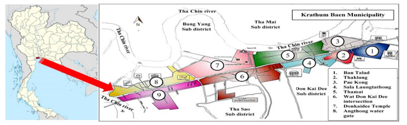
While millions of people around the world die from natural water infections per day because of insufficient wastewater collection systems to cover all communities, 80 percent of used water is still released to the river in Thailand nowadays. As a result, the wastewater management (WWM) behavior of people is critical to water conservation. WWM, on the other hand, was fraught with high expenses and inconvenient installation, and earlier research had paid little attention to it. Thus, this research aims to study the socio-economic, cognition, opinions, and perception of information factors for analysis further of the factors affecting the WWM of people in urban areas, Thailand. This study applied multiple regression analysis from questionnaires survey of nine communities in Krathum Baen municipality, Samut Sakhon Province which is a semi-industrial area, crowded settlement, and risen wastewater unexpectedly along the Tha Chin River. The findings reveal that people in study areas have a moderate level of cognition and opinion toward WWM behavior. Perception of information was the best variable to describe the people's WWM behaviors in urban areas. Addressing the empirical results could contribute to water conservation planning, people engagement, and appropriately promoting WWM behaviors related to urban people.
Citation: Wanjai Lamprom, Surasak Jotaworn, Nuttakit Iamsomboon, Pimnapat Bhumkittipich, Issara Siramaneerat, Anong Rukwong. Exploration of wastewater management behavior for enhancing water conservation in urban area, Thailand[J]. AIMS Environmental Science, 2022, 9(1): 66-82. doi: 10.3934/environsci.2022005
While millions of people around the world die from natural water infections per day because of insufficient wastewater collection systems to cover all communities, 80 percent of used water is still released to the river in Thailand nowadays. As a result, the wastewater management (WWM) behavior of people is critical to water conservation. WWM, on the other hand, was fraught with high expenses and inconvenient installation, and earlier research had paid little attention to it. Thus, this research aims to study the socio-economic, cognition, opinions, and perception of information factors for analysis further of the factors affecting the WWM of people in urban areas, Thailand. This study applied multiple regression analysis from questionnaires survey of nine communities in Krathum Baen municipality, Samut Sakhon Province which is a semi-industrial area, crowded settlement, and risen wastewater unexpectedly along the Tha Chin River. The findings reveal that people in study areas have a moderate level of cognition and opinion toward WWM behavior. Perception of information was the best variable to describe the people's WWM behaviors in urban areas. Addressing the empirical results could contribute to water conservation planning, people engagement, and appropriately promoting WWM behaviors related to urban people.

| [1] | UN-HABITAT (2011) Cities and climate change: Global report on human settlement. London. Earthscan. |
| [2] | Brockwell E, Elofsson K (2020) The role of water quality for local environmental policy implementation. J Environm Plann Man 63: 1001-1021. |
| [3] | Russell SV, Knoeri C (2020) Exploring the psychosocial and behavioural determinants of household water conservation and intention. Int J Water Resour Dev 36: 940-955. |
| [4] | UNICEF (2010) Progress on Sanitation and Drinking Water. World Health Organization and UNICEF, France: WHO-Press. |
| [5] | Pollution Control Department (PCD) (2012), Pollution Control Department. Handbook of wastewater management for households. Community wastewater Bureau of Water Quality Management Pollution Control Department, Bangkok. Available from: http://wqm.pcd.go.th/water |
| [6] | Sapci O, Considine T (2014) The link between environmental attitudes and energy consumption behavior. J Beh Exp Econ 52: 29-34. |
| [7] | Iamsomboon N, Jeerapattanatorn P, Duangpatra P. (2019) E-SCI Knowledge Framework in Community Water Resources Management. EnvironmentAsia 12. |
| [8] | Krathum Baen District Administrative Committee. 4-year district development plan (2018–2021) Krathum Baen District Samut Sakhon Province Krathum Baen District, Samut Sakhon. In Press. |
| [9] | Mavriou Z, Kazakis N, Pliakas FK (2019) Assessment of groundwater vulnerability in the north aquifer area of Rhodes Island using the GALDIT method and GIS. Environments 6: 56. |
| [10] | Ludwig W, Dumont E, Meybeck M, et al. (2009) River discharges of water and nutrients to the Mediterranean and Black Sea: major drivers for ecosystem changes during past and future decades? Progress in oceanography 80: 199-217. |
| [11] | Auesuwanna P (2000) Wastewater Management and Factors Influencing Wastewater Management of Housing Estate Projects Requiring EIA in Bangkok Metropolitan Region. Master's thesis, Mahidol University, Bangkok, Thailand. In Press. |
| [12] | Sattayapan A. (2001) Guidelines for Wastewater Management in the Housing Subdivision in Bangkok. Master's thesis, Chulalongkorn University, Bangkok. ISBN 974-03-1009-5 |
| [13] | Chankaew K (2004) Environmental Science. 6th edition, Bangkok: Kasetsart University Press. |
| [14] | Moonpruek P (2003) Environmental Health. 3rd Edition, Bangkok: Sigma Design Graphics Company Limited. |
| [15] | Kayode OF, Luethi C, Rene ER. (2018) Management recommendations for improving decentralized wastewater treatment by the food and beverage industries in Nigeria. Environments 5: 41. |
| [16] | Gray S, Booker N (2003) Wastewater services for small communities. Water Sci Technol 47: 65-71. |
| [17] | Sarikaya HZ, Sevimli MF, Koyuncu I, et al. (2004) Joint operation of small wastewater treatment plants in southern Turkey. Water Sci Technol 48: 69-76. |
| [18] | Ajzen I (1991) The theory of planned behavior. Organ Behav Hum Dec 50: 179-211. |
| [19] | Wang MY, Lin M. (2020) Intervention strategies on the wastewater treatment behavior of swine farmers: An extended model of the theory of planned behavior. Sustainability 12: 6906. |
| [20] | Sujaritpong S, Nitivattananon V (2009) Factors influencing wastewater management performance: case study of housing estates in suburban Bangkok, Thailand. J Environ Manage 90: 455-465. |
| [21] | Nampim P (2015) the Relationship between Riverbank Community Lifestyle and Sewage Behavior through Thachin River. Acad Service journal Princ Songkla Univ 26: 3. |
| [22] | Suthirak A, Boonyaway S, Dampin N (2017) Wastewater Management Suitability of Settlement Pattern of Thahin River Community: Case Study in the Middle Thachin River Area. Acad Service journal Princ Songkla Univ 28: 150–162. |
| [23] | Mallor K (2012) Household perception and behavior towards solving pollution problems of Tha Chin River. Environ Health J. 15: 1. |
| [24] | Ngamwong W (2002) Behavioral Change on Use Water Supply and Wastewater Treatment in Uttaradit Municipality, Changwat Uttaradit. Master of Science (Environmental Science) Environmental Science, College of Environment. Kasetsart University, Bangkok. In Press. |
| [25] | Sirivachiraporn A (2007) Factors Affecting Existence of Traditional Community Settlements Pak Khlong Wat Pradu Samut Songkhram and Ratchaburi provinces. Master's thesis Department of Urban Planning, Chulalongkorn University. In Press |
| [26] | Karmoker J, Kumar S, Pal BK, et al. (2018) Characterization of wastewater from Jhenaidah municipality area, Bangladesh: A combined physico-chemical and statistical approach. AIMS Environ Sci 5: 389-401. |
| [27] | Best JW (1997) Research in Education. 3rd ed. Englewood Cliffs, New Jersey: Prentice Hall, Inc |
Figures(3) / Tables(7)

Wanjai Lamprom, Surasak Jotaworn, Nuttakit Iamsomboon, Pimnapat Bhumkittipich, Issara Siramaneerat, Anong Rukwong. Exploration of wastewater management behavior for enhancing water conservation in urban area, Thailand[J]. AIMS Environmental Science, 2022, 9(1): 66-82. doi: 10.3934/environsci.2022005


 DownLoad: