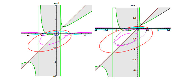
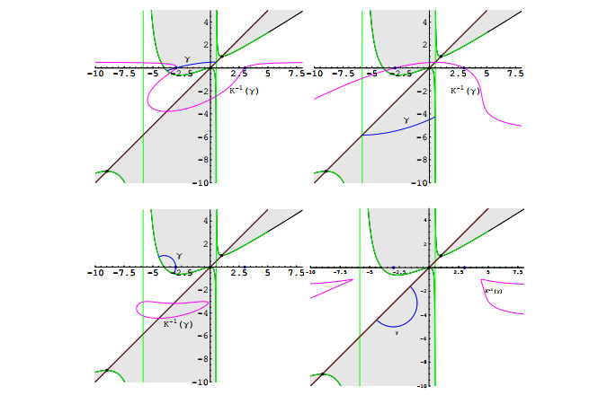
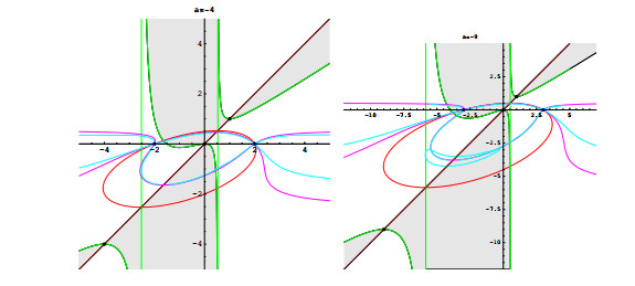
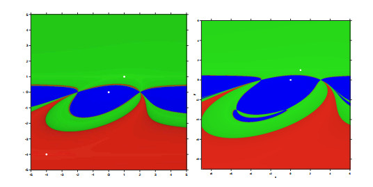
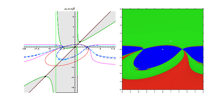
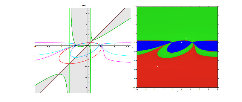
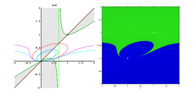
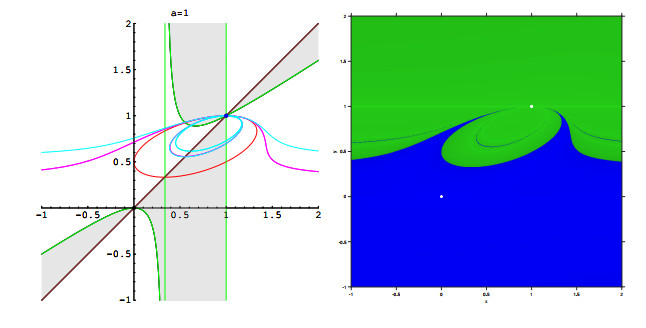
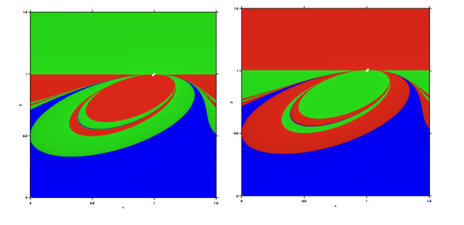
Qualitative analysis of iterative methods with memory has been carried out a few years ago. Most of the papers published in this context analyze the behaviour of schemes on quadratic polynomials. In this paper, we accomplish a complete dynamical study of an iterative method with memory, the Kurchatov scheme, applied on a family of cubic polynomials. To reach this goal we transform the iterative scheme with memory into a discrete dynamical system defined on $ \mathbf{R}^2 $. We obtain a complete description of the dynamical planes for every value of parameter of the family considered. We also analyze the bifurcations that occur related with the number of fixed points. Finally, the dynamical results are summarized in a parameter line. As a conclusion, we obtain that this scheme is completely stable for cubic polynomials since the only attractors that appear for any value of the parameter, are the roots of the polynomial.
Citation: Beatriz Campos, Alicia Cordero, Juan R. Torregrosa, Pura Vindel. Dynamical analysis of an iterative method with memory on a family of third-degree polynomials[J]. AIMS Mathematics, 2022, 7(4): 6445-6466. doi: 10.3934/math.2022359
Qualitative analysis of iterative methods with memory has been carried out a few years ago. Most of the papers published in this context analyze the behaviour of schemes on quadratic polynomials. In this paper, we accomplish a complete dynamical study of an iterative method with memory, the Kurchatov scheme, applied on a family of cubic polynomials. To reach this goal we transform the iterative scheme with memory into a discrete dynamical system defined on $ \mathbf{R}^2 $. We obtain a complete description of the dynamical planes for every value of parameter of the family considered. We also analyze the bifurcations that occur related with the number of fixed points. Finally, the dynamical results are summarized in a parameter line. As a conclusion, we obtain that this scheme is completely stable for cubic polynomials since the only attractors that appear for any value of the parameter, are the roots of the polynomial.

| [1] | V. A. Kurchatov, On a method of linear interpolation for the solution of funcional equations (Russian), Dolk. Akad. Nauk SSSR, 198 (1971), 524–526. Translation in Soviet Math. Dolk. 12, 835–838. |
| [2] | M. Petković, B. Neta, L. Petković, J. Džunić, Multipoint Methods for Solving Nonlinear Equations, Boston: Academic Press, 2013. |
| [3] |
A. Cordero, T. Lotfi, P. Bakhtiari, J. R. Torregrosa, An efficient two-parametric family with memory for nonlinear equations, Numer. Algorithms, 68 (2015), 323–335. https://doi.org/10.1016/j.worlddev.2014.11.009 doi: 10.1016/j.worlddev.2014.11.009

|
| [4] |
A. Cordero, T. Lotfi, J. R. Torregrosa, P. Assari, S. Taher-Khani, Some new bi-accelerator two-point method for solving nonlinear equations, J. Comput. Appl. Math., 35 (2016), 251–267. https://doi.org/10.1002/sim.6628 doi: 10.1002/sim.6628
|
| [5] |
X. Wang, T. Zhang, Y. Qin, Efficient two-step derivative-free iterative methods with memory and their dynamics, Int. J. Comput. Math., 93 (2016), 1423–1446. https://doi.org/10.1080/00207160.2015.1056168 doi: 10.1080/00207160.2015.1056168
|
| [6] |
P. Bakhtiari, A. Cordero, T. Lotfi, K. Mahdiani, J. R. Torregrosa, Widening basins of attraction of optimal iterative methods for solving nonlinear equations, Nonlinear Dynam., 87 (2017), 913–938. https://doi.org/10.1007/s11071-016-3089-2 doi: 10.1007/s11071-016-3089-2
|
| [7] |
C. L. Howk, J. L. Hueso, E. Martínez, C. Teruel, A class of efficient high-order iterative methods with memory for nonlinear equations and their dynamics, Math. Meth. Appl. Sci., 41 (2018), 7263–7282. https://doi.org/10.1002/mma.4821 doi: 10.1002/mma.4821
|
| [8] |
B. Campos, A. Cordero, J. R. Torregrosa, P. Vindel, A multidimensional dynamical approach to iterative methods with memory, Appl. Math. Comput., 271 (2015), 701–715. https://doi.org/10.1016/j.amc.2015.09.056 doi: 10.1016/j.amc.2015.09.056
|
| [9] |
B. Campos, A. Cordero, J. R. Torregrosa, P. Vindel, Stability of King's family of iterative methods with memory, Comput. Appl. Math., 318 (2017), 504–514. https://doi.org/10.1016/j.cam.2016.01.035 doi: 10.1016/j.cam.2016.01.035
|
| [10] | N. Choubey, A. Cordero, J. P. Jaiswal, J. R. Torregrosa, Dynamical techniques for analyzing iterative schemes with memory, Complexity, 2018 (2018), Article ID 1232341, 13 pages. |
| [11] |
F. I. Chicharro, A. Cordero, N. Garrido, J. R. Torregrosa, Stability and applicability of iterative methods with memory, J. Math. Chem., 57 (2019), 1282–1300. https://doi.org/10.1007/s10910-018-0952-z doi: 10.1007/s10910-018-0952-z
|
| [12] |
F. I. Chicharro, A. Cordero, N. Garrido, J. R. Torregrosa, On the choice of the best members of the Kim family and the improvement of its convergence, Math. Meth. Appl. Sci., 43 (2020), 8051–8066. https://doi.org/10.1002/mma.6014 doi: 10.1002/mma.6014
|
| [13] | F. I. Chicharro, A. Cordero, N. Garrido, J. R. Torregrosa, Impact on stability by the use of memory in Traub-type schemes, Mathematics, 8 (2020), 274. |
| [14] |
A. Cordero, F. Soleymani, J. R. Torregrosa, F. K. Haghani, A family of Kurchatov-type methods and its stability, Appl. Math. Comput., 294 (2017), 264–279. https://doi.org/10.1016/j.amc.2016.09.021 doi: 10.1016/j.amc.2016.09.021
|
| [15] | R. C. Robinson, An Introduction to Dynamical Systems, Continous and Discrete, Providence: Americal Mathematical Society, 2012. |
| [16] |
G. Bischi, L. Gardini, C. Mira, Plane maps with denomiator I. Some generic properties, Int. J. Bifurcations Chaos, 9 (1999), 119–153. https://doi.org/10.2307/605565 doi: 10.2307/605565
|
| [17] |
G. Bischi, L. Gardini, C. Mira, Plane maps with denomiator II. Non invertible maps with simple focal points, Int. J. Bifurcations Chaos, 13 (2003), 2253–2277. https://doi.org/10.1142/S021812740300793X doi: 10.1142/S021812740300793X
|
| [18] |
G. Bischi, L. Gardini, C. Mira, Plane maps with denomiator III. Non simple focal points and related bifurcations, Int. J. Bifurcations Chaos, 15 (2005), 451–496. https://doi.org/10.1142/S0218127405012314 doi: 10.1142/S0218127405012314
|
| [19] | G. Bischi, L. Gardini, C. Mira, New phenomena related to the presence of focal points in two dimensional maps, J. Ann. Math. Salesiane, (special issue Proceedings ECIT98), 13 (1999), 81–90. |
| [20] |
A. Garijo, X. Jarque, Global dynamics of the real secant method, Nonlinearity, 32 (2019), 4557–4578. https://doi.org/10.1088/1361-6544/ab2f55 doi: 10.1088/1361-6544/ab2f55
|
| [21] |
A. Garijo, X. Jarque, The secant map applied to a real polynomial with multiple roots, Discrete Cont. Dyn-A., 40 (2020), 6783–6794. https://doi.org/10.3934/dcds.2020133 doi: 10.3934/dcds.2020133
|
| [22] | L. Gardini, G. Bischi, D. Fournier-Prunaret, Basin boundaries and focal points in a map coming from Bairstow's method, Chaos, 9 (1999), 367–380. |
| [23] | M. R. Ferchichi, I. Djellit, On some properties of focal points, Discrete Dyn. Nat. Soc., 2009 (2009), Article ID 646258, 11 pages. |
| [24] | G. Bischi, L. Gardini, C. Mira, Contact bifurcations related to critical sets and focal points in iterated maps of the plane, Proceedings of the International Workshop Future Directions in Difference Equations, (2011), 15–50. |
| [25] | N. Pecora, F. Tramontana, Maps with vanishing denominator and their applications, Front. Appl. Math. Stat., 2 (2016), 12 pages. |

Figures(14)

Beatriz Campos, Alicia Cordero, Juan R. Torregrosa, Pura Vindel. Dynamical analysis of an iterative method with memory on a family of third-degree polynomials[J]. AIMS Mathematics, 2022, 7(4): 6445-6466. doi: 10.3934/math.2022359


 DownLoad: