


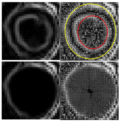
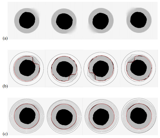
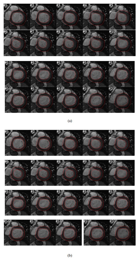
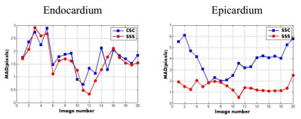
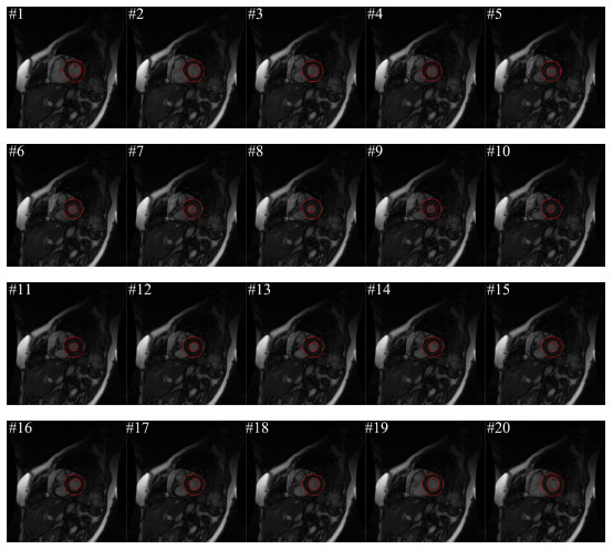
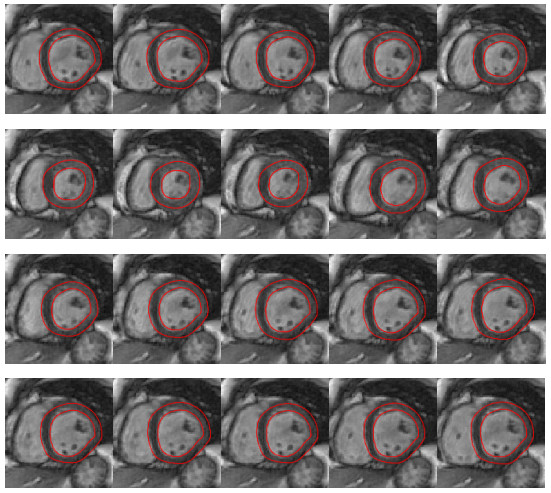
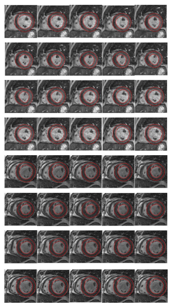
Delineation of the boundaries of the Left Ventricle (LV) in cardiac Magnetic Resonance Images (MRI) is a hot topic due to its important diagnostic power. In this paper, an approach is proposed to extract the LV in a sequence of MR images. In the proposed paper, all images in the sequence are segmented simultaneously and the shape of the LV in each image is supposed to be similar to that of the LV in nearby images in the sequence. We coined the novel shape similarity constraint, and it is called sequential shape similarity (SSS in short). The proposed segmentation method takes the Active Contour Model as the base model and our previously proposed Gradient Vector Convolution (GVC) external force is also adopted. With the SSS constraint, the snake contour can accurately delineate the LV boundaries. We evaluate our method on two cardiac MRI datasets and the Mean Absolute Distance (MAD) metric and the Hausdorff Distance (HD) metric demonstrate that the proposed approach has good performance on segmenting the boundaries of the LV.
Citation: Ke Bi, Yue Tan, Ke Cheng, Qingfang Chen, Yuanquan Wang. Sequential shape similarity for active contour based left ventricle segmentation in cardiac cine MR image[J]. Mathematical Biosciences and Engineering, 2022, 19(2): 1591-1608. doi: 10.3934/mbe.2022074
| [1] | Rajalakshmi Manoharan, Reenu Rani, Ali Moussaoui . Predator-prey dynamics with refuge, alternate food, and harvesting strategies in a patchy habitat. Mathematical Biosciences and Engineering, 2025, 22(4): 810-845. doi: 10.3934/mbe.2025029 |
| [2] | Fang Liu, Yanfei Du . Spatiotemporal dynamics of a diffusive predator-prey model with delay and Allee effect in predator. Mathematical Biosciences and Engineering, 2023, 20(11): 19372-19400. doi: 10.3934/mbe.2023857 |
| [3] | Hongqiuxue Wu, Zhong Li, Mengxin He . Dynamic analysis of a Leslie-Gower predator-prey model with the fear effect and nonlinear harvesting. Mathematical Biosciences and Engineering, 2023, 20(10): 18592-18629. doi: 10.3934/mbe.2023825 |
| [4] | Xin-You Meng, Yu-Qian Wu . Bifurcation analysis in a singular Beddington-DeAngelis predator-prey model with two delays and nonlinear predator harvesting. Mathematical Biosciences and Engineering, 2019, 16(4): 2668-2696. doi: 10.3934/mbe.2019133 |
| [5] | Ting Yu, Qinglong Wang, Shuqi Zhai . Exploration on dynamics in a ratio-dependent predator-prey bioeconomic model with time delay and additional food supply. Mathematical Biosciences and Engineering, 2023, 20(8): 15094-15119. doi: 10.3934/mbe.2023676 |
| [6] | Sourav Kumar Sasmal, Jeet Banerjee, Yasuhiro Takeuchi . Dynamics and spatio-temporal patterns in a prey–predator system with aposematic prey. Mathematical Biosciences and Engineering, 2019, 16(5): 3864-3884. doi: 10.3934/mbe.2019191 |
| [7] | Yuanfu Shao . Bifurcations of a delayed predator-prey system with fear, refuge for prey and additional food for predator. Mathematical Biosciences and Engineering, 2023, 20(4): 7429-7452. doi: 10.3934/mbe.2023322 |
| [8] | Rongjie Yu, Hengguo Yu, Chuanjun Dai, Zengling Ma, Qi Wang, Min Zhao . Bifurcation analysis of Leslie-Gower predator-prey system with harvesting and fear effect. Mathematical Biosciences and Engineering, 2023, 20(10): 18267-18300. doi: 10.3934/mbe.2023812 |
| [9] | Christian Cortés García, Jasmidt Vera Cuenca . Impact of alternative food on predator diet in a Leslie-Gower model with prey refuge and Holling Ⅱ functional response. Mathematical Biosciences and Engineering, 2023, 20(8): 13681-13703. doi: 10.3934/mbe.2023610 |
| [10] | Manoj K. Singh, Brajesh K. Singh, Poonam, Carlo Cattani . Under nonlinear prey-harvesting, effect of strong Allee effect on the dynamics of a modified Leslie-Gower predator-prey model. Mathematical Biosciences and Engineering, 2023, 20(6): 9625-9644. doi: 10.3934/mbe.2023422 |
Delineation of the boundaries of the Left Ventricle (LV) in cardiac Magnetic Resonance Images (MRI) is a hot topic due to its important diagnostic power. In this paper, an approach is proposed to extract the LV in a sequence of MR images. In the proposed paper, all images in the sequence are segmented simultaneously and the shape of the LV in each image is supposed to be similar to that of the LV in nearby images in the sequence. We coined the novel shape similarity constraint, and it is called sequential shape similarity (SSS in short). The proposed segmentation method takes the Active Contour Model as the base model and our previously proposed Gradient Vector Convolution (GVC) external force is also adopted. With the SSS constraint, the snake contour can accurately delineate the LV boundaries. We evaluate our method on two cardiac MRI datasets and the Mean Absolute Distance (MAD) metric and the Hausdorff Distance (HD) metric demonstrate that the proposed approach has good performance on segmenting the boundaries of the LV.
Time inconsistency in dynamic decision making is often observed in social systems and daily life. Motivated by practical applications, especially in mathematical economics and finance, time-inconsistency control problems have recently attracted considerable research interest and efforts attempting to seek equilibrium, instead of optimal controls. At a conceptual level, the idea is that a decision made by the controller at every instant of time is considered as a game against all the decisions made by the future incarnations of the controller. An "equilibrium" control is therefore one such that any deviation from it at any time instant will be worse off. The study on time inconsistency by economists can be dated back to Stroz [1] and Phelps [2,3] in models with discrete time (see [4] and [5] for further developments), and adapted by Karp [6,7], and by Ekeland and Lazrak [8,9,10,11,12,13] to the case of continuous time. In the LQ control problems, Yong [14] studied a time-inconsistent deterministic model and derived equilibrium controls via some integral equations.
It is natural to study time inconsistency in the stochastic models. Ekeland and Pirvu [15] studied the non-exponential discounting which leads to time inconsistency in an agent's investment-consumption policies in a Merton model. Grenadier and Wang [16] also studied the hyperbolic discounting problem in an optimal stopping model. In a Markovian systems, Björk and Murgoci [17] proposed a definition of a general stochastic control problem with time inconsistent terms, and proposed some sufficient condition for a control to be solution by a system of integro-differential equations. They constructed some solutions for some examples including an LQ one, but it looks very hard to find not-to-harsh condition on parameters to ensure the existence of a solution. Björk, Murgoci and Zhou [18] also constructed an equilibrium for a mean-variance portfolio selection with state-dependent risk aversion. Basak and Chabakauri [19] studied the mean-variance portfolio selection problem and got more details on the constructed solution. Hu, Jin and Zhou [20,21] studied the general LQ control problem with time inconsistent terms in a non-Markovian system and constructed an unique equilibrium for quite general LQ control problem, including a non-Markovian system.
To the best of our knowledge, most of the time-inconsistent problems are associated with the control problems though we use the game formulation to define its equilibrium. In the problems of game theory, the literatures about time inconsistency is little [22,23]. However, the definitions of equilibrium strategies in the above two papers are based on some corresponding control problems like before. In this paper, we formulate a general stochastic LQ differential game, where the objective functional of each player include both a quadratic term of the expected state and a state-dependent term. These non-standard terms each introduces time inconsistency into the problem in somewhat different ways. We define our equilibrium via open-loop controls. Then we derive a general sufficient condition for equilibrium strategies through a system of forward-backward stochastic differential equations (FBSDEs). An intriguing feature of these FBSDEs is that a time parameter is involved; so these form a flow of FBSDEs. When the state process is scalar valued and all the coefficients are deterministic functions of time, we are able to reduce this flow of FBSDEs into several Riccati-like ODEs. Comparing to the ODEs in [20], though the state process is scalar valued, the unknowns are matrix-valued because of two players. Therefore, such ODEs are harder to solve than those of [20]. Under some more stronger conditions, we obtain explicitly an equilibrium strategy, which turns out to be a linear feedback. We also prove that the equilibrium strategy we obtained is unique.
The rest of the paper is organized as follows. The next section is devoted to the formulation of our problem and the definition of equilibrium strategy. In Section 3, we apply the spike variation technique to derive a flow of FBSEDs and a sufficient condition of equilibrium strategies. Based on this general results, we solve in Section 4 the case when the state is one dimensional and all the coefficients are deterministic. The uniqueness of such equilibrium strategy is also proved in this section.
Let T>0 be the end of a finite time horizon, and let (Wt)0≤t≤T=(W1t,...,Wdt)0≤t≤T be a d-dimensional Brownian motion on a probability space (Ω,F,P). Denote by (Ft) the augmented filtration generated by (Wt).
Let Sn be the set of symmetric n×n real matrices; L2F(Ω,Rl) be the set of square-integrable random variables; L2F(t,T;Rn) be the set of {Fs}s∈[t,T]-adapted square-integrable processes; and L2F(Ω;C(t,T;Rn)) be the set of continuous {Fs}s∈[t,T]-adapted square-integrable processes.
We consider a continuous-time, n-dimensional nonhomogeneous linear controlled system:
| dXs=[AsXs+B′1,su1,s+B′2,su2,s+bs]ds+d∑j=1[CjsXs+Dj1,su1,s+Dj2,su2,s+σjs]dWjs,X0=x0. | (2.1) |
Here A is a bounded deterministic function on [0,T] with value in Rn×n. The other parameters B1,B2,C,D1,D2 are all essentially bounded adapted processes on [0,T] with values in Rl×n,Rl×n,Rn×n,Rn×l,Rn×l, respectively; b and σj are stochastic processes in L2F(0,T;Rn). The processes ui∈L2F(0,T;Rl), i=1,2 are the controls, and X is the state process valued in Rn. Finally, x0∈Rn is the initial state. It is obvious that for any controls ui∈L2F(0,T;Rl), i=1,2, there exists a unique solution X∈L2F(Ω,C(0,T;Rn)).
As time evolves, we need to consider the controlled system starting from time t∈[0,T] and state xt∈L2Ft(Ω;Rn):
| dXs=[AsXs+B′1,su1,s+B′2,su2,s+bs]ds+d∑j=1[CjsXs+Dj1,su1,s+Dj2,su2,s+σjs]dWjs,Xt=xt. | (2.2) |
For any controls ui∈L2F(0,T;Rl), i=1,2, there exists a unique solution Xt,xt,u1,u2∈L2F(Ω,C(0,T;Rn)).
We consider a two-person differential game problem. At any time t with the system state Xt=xt, the i-th (i=1,2) person's aim is to minimize her cost (if maximize, we can times the following function by −1):
| Ji(t,xt;u1,u2)=12Et∫Tt[⟨Qi,sXs,Xs⟩+⟨Ri,sui,s,ui,s⟩]ds+12Et[⟨GiXT,XT⟩]−12⟨hiEt[XT],Et[XT]⟩−⟨λixt+μi,Et[XT]⟩ | (2.3) |
over u1,u2∈L2F(t,T;Rl), where X=Xt,xt,u1,u2, and Et[⋅]=E[⋅|Ft]. Here, for i=1,2, Qi and Ri are both given essentially bounded adapted process on [0,T] with values in Sn and Sl, respectively, Gi,hi,λi,μi are all constants in Sn, Sn, Rn×n and Rn, respectively. Furthermore, we assume that Qi,Ri are non-negative definite almost surely and Gi are non-negative definite.
Given a control pair (u∗1,u∗2). For any t∈[0,T),ϵ>0, and v1,v2∈L2Ft(Ω,Rl), define
| ut,ϵ,vii,s=u∗i,s+vi1s∈[t,t+ϵ),s∈[t,T], i=1,2. | (2.4) |
Because each person at time t>0 wants to minimize his/her cost as we claimed before, we have
Definition 2.1. Let (u∗1,u∗2)∈L2F(0,T;Rl)×L2F(0,T;Rl) be a given strategy pair, and let X∗ be the state process corresponding to (u∗1,u∗2). The strategy pair (u∗1,u∗2) is called an equilibrium if
| limϵ↓0J1(t,X∗t;ut,ϵ,v11,u∗2)−J1(t,X∗t;u∗1,u∗2)ϵ≥0, | (2.5) |
| limϵ↓0J2(t,X∗t;u∗1,ut,ϵ,v22)−J2(t,X∗t;u∗1,u∗2)ϵ≥0, | (2.6) |
where ut,ϵ,vii,i=1,2 are defined by (2.4), for any t∈[0,T) and v1,v2∈L2Ft(Ω,Rl).
Remark. The above definition means that, in each time t, the equilibrium is a static Nash equilibrium in a corresponding game.
Let (u∗1,u∗2) be a fixed strategy pair, and let X∗ be the corresponding state process. For any t∈[0,T), as a similar arguments of Theorem 5.1 in pp. 309 of [24], defined in the time interval [t,T], there exist adapted processes (pi(⋅;t),(kji(⋅;t)j=1,2,...,d))∈L2F(t,T;Rn)×(L2F(t,T;Rn))d and (Pi(⋅;t),(Kji(⋅;t)j=1,2,...,d))∈L2F(t,T;Sn)×(L2F(t,T;Sn))d for i=1,2 satisfying the following equations:
| {dpi(s;t)=−[A′spi(s;t)+∑dj=1(Cjs)′kji(s;t)+Qi,sX∗s]ds+∑dj=1kji(s;t)dWjs,s∈[t,T],pi(T;t)=GiX∗T−hiEt[X∗T]−λiX∗t−μi, | (3.1) |
| {dPi(s;t)=−{A′sPi(s;t)+Pi(s;t)As+Qi,s+∑dj=1[(Cjs)′Pi(s;t)Cjs+(Cjs)′Kji(s;t)+Kji(s;t)Cjs]}ds+∑dj=1Kji(s;t)dWji,s∈[t,T],Pi(T;t)=Gi, | (3.2) |
for i=1,2. From the assumption that Qi and Gi are non-negative definite, it follows that Pi(s;t) are non-negative definite for i=1,2.
Proposition 1. For any t∈[0,T),ϵ>0, and v1,v2∈L2Ft(Ω,Rl), define ut,ϵ,vii,i=1,2 by (2.4). Then
| J1(t,X∗t;ut,ϵ,v11,u∗2)−J1(t,X∗t;u∗1,u∗2)=Et∫t+ϵt{⟨Λ1(s;t),v1⟩+12⟨H1(s;t)v1,v1⟩}ds+o(ϵ), | (3.3) |
| J2(t,X∗t;u∗1,ut,ϵ,v22)−J2(t,X∗t;u∗1,u∗2)=Et∫t+ϵt{⟨Λ2(s;t),v2⟩+12⟨H2(s;t)v2,v2⟩}ds+o(ϵ), | (3.4) |
where Λi(s;t)=Bi,spi(s;t)+∑dj=1(Dji,s)′kji(s;t)+Ri,su∗i,s and Hi(s;t)=Ri,s+∑dj=1(Dji,s)′Pi(s;t)Dji,s for i=1,2.
Proof. Let Xt,ϵ,v1,v2 be the state process corresponding to ut,ϵ,vii,i=1,2. Then by standard perturbation approach (cf. [20,25] or pp. 126-128 of [24]), we have
| Xt,ϵ,v1,v2s=X∗s+Yt,ϵ,v1,v2s+Zt,ϵ,v1,v2s,s∈[t,T], | (3.5) |
where Y≡Yt,ϵ,v1,v2 and Z≡Zt,ϵ,v1,v2 satisfy
| {dYs=AsYsds+∑dj=1[CjsYs+Dj1,sv11s∈[t,t+ϵ)+Dj2,sv21s∈[t,t+ϵ)]dWjs,s∈[t,T],Yt=0, | (3.6) |
| {dZs=[AsZs+B′1,sv11s∈[t,t+ϵ)+B′2,sv21s∈[t,t+ϵ)]ds+∑dj=1CjsZsdWjs,s∈[t,T],Zt=0. | (3.7) |
Moreover, by Theorem 4.4 in [24], we have
| Et[sups∈[t,T)|Ys|2]=O(ϵ),Et[sups∈[t,T)|Zs|2]=O(ϵ2). | (3.8) |
With A being deterministic, it follows from the dynamics of Y that, for any s∈[t,T], we have
| Et[Ys]=∫stEt[AsYτ]dτ=∫stAsEt[Yτ]dτ. | (3.9) |
Hence we conclude that
| Et[Ys]=0s∈[t,T]. | (3.10) |
By these estimates, we can calculate
| Ji(t,X∗t;ut,ϵ,v11,ut,ϵ,v22)−Ji(t,X∗t;u∗1,u∗2)=12Et∫Tt[<Qi,s(2X∗s+Ys+Zs),Ys+Zs>+<Ri,s(2u∗i+vi),vi>1s∈[t,t+ϵ)]ds+Et[<GiX∗T,YT+ZT>]+12Et[<Gi(YT+ZT),YT+ZT>]−<hiEt[X∗T]+λiX∗t+μi,Et[YT+ZT]>−12<hiEt[YT+ZT],Et[YT+ZT]>=12Et∫Tt[<Qi,s(2X∗s+Ys+Zs),Ys+Zs>+<Ri,s(2u∗i+vi),vi>1s∈[t,t+ϵ)]ds+Et[<GiX∗T−hiEt[X∗T]−λiX∗t−μi,YT+ZT>+12<Gi(YT+ZT),YT+ZT>]+o(ϵ). | (3.11) |
Recalling that (pi(⋅;t),ki(⋅;t)) and (Pi(⋅;t),Ki(⋅;t)) solve, respectively, BSDEs (3.1) and (3.2) for i=1,2, we have
| Et[<GiX∗T−hiEt[X∗T]−λiX∗t−μi,YT+ZT>]=Et[<pi(T;t),YT+ZT>]=Et[∫Ttd<pi(s;t),Ys+Zs>]=Et∫Tt[<pi(s;t),As(Ys+Zs)+B′1,sv11s∈[t,t+ϵ)+B′2,sv21s∈[t,t+ϵ)>−<A′spi(s;t)+d∑j=1(Cjs)′kji(s;t)+Qi,sX∗s,Ys+Zs>+d∑j=1<kji(s;t),Cjs(Ys+Zs)+Dj1,sv11s∈[t,t+ϵ)+Dj2,sv21s∈[t,t+ϵ)>]ds=Et∫Tt[<−Qi,sX∗s>+⟨B1,spi(s;t)+d∑j=1(Dj1,s)′kji(s;t),v11s∈[t,t+ϵ)⟩+⟨B2,spi(s;t)+d∑j=1(Dj2,s)′kji(s;t),v21s∈[t,t+ϵ)⟩]ds | (3.12) |
and
| Et[12<Gi(YT+ZT),YT+ZT>]=Et[12<Pi(T;t)(YT+ZT),YT+ZT>]=Et[∫Ttd<Pi(s;t)(Ys+Zs),Ys+Zs>]=Et∫Tt{<Pi(s;t)(Ys+Zs),As(Ys+Zs)+B′1,sv11s∈[t,t+ϵ)+B′2,sv21s∈[t,t+ϵ)>+<Pi(s;t)[As(Ys+Zs)+B′1,sv11s∈[t,t+ϵ)+B′2,sv21s∈[t,t+ϵ)],Ys+Zs>−<[A′sPi(s;t)+Pi(s;t)As+Qi,s+d∑j=1((Cjs)′Pi(s;t)Cjs+(Cjs)′Kji(s;t)+Kji(s;t)Cjs)](Ys+Zs),Ys+Zs>+d∑j=1<Kji(s;t)(Ys+Zs),Cjs(Ys+Zs)+Dj1,sv11s∈[t,t+ϵ)+Dj2,sv21s∈[t,t+ϵ)>+d∑j=1<Kji(s;t)[Cjs(Ys+Zs)+Dj1,sv11s∈[t,t+ϵ)+Dj2,sv21s∈[t,t+ϵ)],Ys+Zs>+d∑j=1<Pi(s;t)[Cjs(Ys+Zs)+Dj1,sv11s∈[t,t+ϵ)+Dj2,sv21s∈[t,t+ϵ)],Cjs(Ys+Zs)+Dj1,sv11s∈[t,t+ϵ)+Dj2,sv21s∈[t,t+ϵ)>}ds=Et∫Tt[−<Qi,s(Ys+Zs),Ys+Zs>+d∑j=1<Pi(s;t)[Dj1,sv1+Dj2,sv2],Dj1,sv1+Dj2,sv2>1s∈[t,t+ϵ)]ds+o(ϵ) | (3.13) |
Combining (3.11)-(3.13), we have
| Ji(t,X∗t;ut,ϵ,v11,ut,ϵ,v22)−Ji(t,X∗t;u∗1,u∗2)=Et∫Tt[12<Ri,s(2u∗i+vi),vi>1s∈[t,t+ϵ)+⟨B1,spi(s;t)+d∑j=1(Dj1,s)′kji(s;t),v11s∈[t,t+ϵ)⟩+⟨B2,spi(s;t)+d∑j=1(Dj2,s)′kji(s;t),v21s∈[t,t+ϵ)⟩+12d∑j=1<Pi(s;t)[Dj1,sv1+Dj2,sv2],Dj1,sv1+Dj2,sv2>1s∈[t,t+ϵ)]ds+o(ϵ). | (3.14) |
Take i=1, we let v2=0, then ut,ϵ,v22=u∗2, from (3.14), we obtain
| J1(t,X∗t;ut,ϵ,v11,u∗2)−J1(t,X∗t;u∗1,u∗2)=Et∫Tt{⟨R1,su∗1+B1,sp1(s;t)+d∑j=1(Dj1,s)′kj1(s;t),v11s∈[t,t+ϵ)⟩+12⟨[R1,s+d∑j=1(Dj1,s)′P1(s;t)Dj1,s]v1,v1⟩}ds=Et∫t+ϵt{<Λ1(s;t),v1>+12<H1(s;t)v1,v1>}ds+o(ϵ). | (3.15) |
This proves (3.3), and similarly, we obtain (3.4).
Because of Ri,s and Pi(s;t),i=1,2 are non-negative definite, Hi(s;t), i=1,2 are also non-negative definite. In view of (3.3)-(3.4), a sufficient condition for an equilibrium is
| Et∫Tt|Λi(s;t)|ds<+∞,lims↓tEt[Λi(s;t)]=0 a.s. ∀t∈[0,T],i=1,2. | (3.16) |
By an arguments similar to the proof of Proposition 3.3 in [21], we have the following lemma:
Lemma 3.1. For any triple of state and control processes (X∗,u∗1,u∗2), the solution to BSDE (3.1) in L2(0,T;Rn)×(L2(0,T;Rn))d satisfies ki(s;t1)=ki(s;t2) for a.e. s≥max{t1,t2},i=1,2. Furthermore, there exist ρi∈L2(0,T;Rl), δi∈L2(0,T;Rl×n) and ξi∈L2(Ω;C(0,T;Rn)), such that
| Λi(s;t)=ρi(s)+δi(s)ξi(t),i=1,2. | (3.17) |
Therefore, we have another characterization for equilibrium strategies:
Proposition 2. Given a strategy pair (u∗1,u∗2)∈L2(0,T;Rl)×L2(0,T;Rl). Denote X∗ as the state process, and (pi(⋅;t),(kji(⋅;t)j=1,2,...,d))∈L2F(t,T;Rn)×(L2F(t,T;Rn))d as the unique solution for the BSDE (3.1), with ki(s)=ki(s;t) according to Lemma 3.1 for i=1,2 respectively. For i=1,2, letting
| Λi(s,t)=Bi,spi(s;t)+d∑j=1(Dj,s)′k(s;t)j+Ri,su∗i,s,s∈[t,T], | (3.18) |
then u∗ is an equilibrium strategy if and only if
| Λi(t,t)=0,a.s.,a.e.t∈[0,T],i=1,2. | (3.19) |
Proof. From (3.17), we have Λ1(s;t)=ρ1(s)+δ1(s)ξ1(t). Since δ1 is essentially bounded and ξ1 is continuous, we have
| limϵ↓0Et[1ϵ∫t+ϵt|δ1(s)(ξ1(s)−ξ1(t))|ds]≤climϵ↓01ϵ∫t+ϵtEt[|ξ1(s)−ξ1(t)|]ds=0, |
and hence
| limϵ↓01ϵ∫t+ϵtEt[Λ1(s;t)]ds=limϵ↓01ϵ∫t+ϵtEt[Λ1(s;s)]ds. |
Therefore, if (3.19) holds, we have
| limϵ↓01ϵ∫t+ϵtEt[Λ1(s;t)]ds=limϵ↓01ϵ∫t+ϵtEt[Λ1(s;s)]ds=0. |
When i=2, we can prove (3.19) similarly.
Conversely, if (3.16) holds, then limϵ↓01ϵ∫t+ϵtEt[Λi(s;s)]ds=0,i=1,2 leading to (3.19) by virtue of Lemma 3.4 of [21].
The following is the main general result for the stochastic LQ differential game with time-inconsistency.
Theorem 3.2. A strategy pair (u∗1,u∗2)∈L2F(0,T;Rl)×L2F(0,T;Rl) is an equilibrium strategy pair if the following two conditions hold for any time t:
(i) The system of SDEs
| {dX∗s=[AsX∗s+B′1,su∗1,s+B′2,su∗2,s+bs]ds+∑dj=1[CjsX∗s+Dj1,su∗1,s+Dj2,su∗2,s+σjs]dWjs,X∗0=x0,dp1(s;t)=−[A′sp1(s;t)+∑dj=1(Cjs)′kj1(s;t)+Q1,sX∗s]ds+∑dj=1kj1(s;t)dWjs,s∈[t,T],p1(T;t)=G1X∗T−h1Et[X∗T]−λ1X∗t−μ1,dp2(s;t)=−[A′sp2(s;t)+∑dj=1(Cjs)′kj2(s;t)+Q2,sX∗s]ds+∑dj=1kj2(s;t)dWjs,s∈[t,T],p2(T;t)=G2X∗T−h2Et[X∗T]−λ2X∗t−μ2, | (3.20) |
admits a solution (X∗,p1,k1,p2,k2);
(ii) Λi(s;t)=Ri,su∗i,s+Bi,spi(s;t)+∑dj=1(Dji,s)′kji(s;t),i=1,2 satisfy condition (3.19).
Proof. Given a strategy pair (u∗1,u∗2)∈L2F(0,T;Rl)×L2F(0,T;Rl) satisfying (i) and (ii), then for any v1,v2∈L2Ft(Ω,Rl), define Λi,Hi,i=1,2 as in Proposition 1. We have
| limϵ↓0J1(t,X∗t;ut,ϵ,v11,u∗2)−J1(t,X∗t;u∗1,u∗2)ϵ=limϵ↓0Et∫t+ϵt{<Λ1(s;t),v1>+12<H1(s;t)v1,v1>}dsϵ≥limϵ↓0Et∫t+ϵt<Λ1(s;t),v1>dsϵ=0, | (3.21) |
proving the first condition of Definition 2.1, and the proof of the second condition is similar.
Theorem 3.2 involve the existence of solutions to a flow of FBSDEs along with other conditions. The system (3.20) is more complicated than system (3.6) in [20]. As declared in [20], "proving the general existence for this type of FBSEs remains an outstanding open problem", it is also true for our system (3.20).
In the rest of this paper, we will focus on the case when n=1. When n=1, the state process X is a scalar-valued rocess evolving by the dynamics
| dXs=[AsXs+B′1,su1,s+B′2,su2,s+bs]ds+[CsXs+D1,su1,s+D2,su2,s+σs]′dWs,X0=x0, | (3.22) |
where A is a bounded deterministic scalar function on [0,T]. The other parameters B,C,D are all essentially bounded and Ft-adapted processes on [0,T] with values in Rl,Rd,Rd×l, respectively. Moreover, b∈L2F(0,T;R) and σ∈L2F(0,T;Rd).
In this case, the adjoint equations for the equilibrium strategy become
| {dpi(s;t)=−[A′spi(s;t)+(Cs)′ki(s;t)+Qi,sX∗s]ds+ki(s;t)′dWs,s∈[t,T],pi(T;t)=GiX∗T−hiEt[X∗T]−λiX∗t−μi, | (3.23) |
| {dPi(s;t)=−[(2As+|Cs|2)Pi(s;t)+2C′sK(s;t)+Qi,s]ds+Ki(s;t)′dWs,s∈[t,T],Pi(T;t)=Gi, | (3.24) |
for i=1,2. For convenience, we also state here the n=1 version of Theorem 3.2:
Theorem 3.3. A strategy pair (u∗1,u∗2)∈L2F(0,T;Rl)×L2F(0,T;Rl) is an equilibrium strategy pair if, for any time t∈[0,T),
(i) The system of SDEs
| {dX∗s=[AsX∗s+B′1,su∗1,s+B′2,su∗2,s+bs]ds+[CsX∗s+D1,su∗1,s+D2,su∗2,s+σs]′dWs,X∗0=x0,dp1(s;t)=−[Asp1(s;t)+(Cs)′k1(s;t)+Q1,sX∗s]ds+k1(s;t)′dWs,s∈[t,T],p1(T;t)=G1X∗T−h1Et[X∗T]−λ1X∗t−μ1,dp2(s;t)=−[Asp2(s;t)+(Cs)′k2(s;t)+Q2,sX∗s]ds+k2(s;t)′dWs,s∈[t,T],p2(T;t)=G2X∗T−h2Et[X∗T]−λ2X∗t−μ2, | (3.25) |
admits a solution (X∗,p1,k1,p2,k2);
(ii) Λi(s;t)=Ri,su∗i,s+Bi,spi(s;t)+(Di,s)′ki(s;t),i=1,2 satisfy condition (3.19).
The unique solvability of (3.25) remains a challenging open problem even for the case n=1. However, we are able to solve this problem when the parameters A,B1,B2,C,D1,D2,b,σ,Q1,Q2,R1 and R2 are all deterministic functions.
Throughout this section we assume all the parameters are deterministic functions of t. In this case, since G1,G2 have been also assumed to be deterministic, the BSDEs (3.24) turns out to be ODEs with solutions Ki≡0 and Pi(s;t)=Gie∫Ts(2Au+|Cu|2)du+∫Tse∫Ts(2Au+|Cu|2)duQi,vdv for i=1,2. Hence, the equilibrium strategy will be characterized through a system of coupled Riccati-type equations.
As in classical LQ control, we attempt to look for a linear feedback equilibrium strategy pair. For such purpose, motivated by [20], given any t∈[0,T], we consider the following process:
| pi(s;t)=Mi,sX∗s−Ni,sEt[X∗s]−Γi,sX∗t+Φi,s,0≤t≤s≤T,i=1,2, | (4.1) |
where Mi,Ni,Γi,Φi are deterministic differentiable functions with ˙Mi=mi,˙Ni=ni,˙Γi=γi and ˙Φi=ϕi for i=1,2. The advantage of this process is to separate the variables X∗s,Et[X∗s] and X∗t in the solutions pi(s;t),i=1,2, thereby reducing the complicated FBSDEs to some ODEs.
For any fixed t, applying Ito's formula to (4.1) in the time variable s, we obtain, for i=1,2,
| dpi(s;t)={Mi,s(AsX∗s+B′1,su∗1,s+B′2,su∗2,s+bs)+mi,sX∗s−Ni,sEt[AsX∗s+B′1,su∗1,s+B′2,su∗2,s+bs]−ni,sEt[X∗s]−γi,sX∗t+ϕi,s}ds+Mi,s(CsX∗s+D1,su∗1,s+D2,su∗2,s+σs)′dWs. | (4.2) |
Comparing the dWs term of dpi(s;t) in (3.25) and (4.2), we have
| ki(s;t)=Mi,s[CsX∗s+D1,su∗1,s+D2,su∗2,s+σs],s∈[t,T],i=1,2. | (4.3) |
Notice that k(s;t) turns out to be independent of t.
Putting the above expressions (4.1) and (4.3) of pi(s;t) and ki(s;t),i=1,2 into (3.19), we have
| Ri,su∗i,s+Bi,s[(Mi,s−Ni,s−Γi,s)X∗s+Φi,s]+D′i,sMi,s[CsX∗s+D1,su∗1,s+D2,su∗2,s+σs]=0,s∈[0,T], | (4.4) |
for i=1,2. Then we can formally deduce
| u∗i,s=αi,sX∗s+βi,s,i=1,2. | (4.5) |
Let Ms=diag(M1,sIl,M2,sIl),Ns=diag(N1,sIl,N2,sIl),Γs=diag(Γ1,sIl,Γ2,sIl),Φs=diag(Φ1,sIl,Φ2,sIl), Rs=diag(R1,s,R2,s),Bs=(B1,sB2,s),Ds=(D1,s,D2,s), u∗s=(u∗1,su∗2,s),αs=(α1,sα2,s) and βs=(β1,sβ2,s). Then from (4.4), we have
| Rsu∗s+[(Ms−Ns−Γs)X∗s+Φs]Bs+MsD′s[CsX∗s+Ds(αsX∗s+βs)+σs]=0,s∈[0,T] | (4.6) |
and hence
| αs=−(Rs+MsD′sDs)−1[(Ms−Ns−Γs)Bs+MsD′sCs], | (4.7) |
| βs=−(Rs+MsD′sDs)−1(ΦsBs+MsD′sσs). | (4.8) |
Next, comparing the ds term of dpi(s;t) in (3.25) and (4.2) (we supress the argument s here), we have
| Mi[AX∗+B′(αX∗+β)+b]+miX∗−Ni{AEt[X∗]+B′Et[αX∗+β]+b}−niEt[X∗]−γiX∗t+ϕi=−[A(MiX∗−NiEt[X∗]−ΓiX∗t+Φi)+MiC′(CX∗+D(αX∗+β)+σ)]. | (4.9) |
Notice in the above that X∗=X∗s and Et[X∗]=Et[X∗s] due to the omission of s. This leads to the following equations for Mi,Ni,Γi,Φi:
| {˙Mi=−(2A+|C|2)Mi−Qi+Mi(B′+C′D)(R+MD′D)−1[(M−N−Γ)B+MD′C],s∈[0,T],Mi,T=Gi; | (4.10) |
| {˙Ni=−2ANi+NiB′(R+MD′D)−1[(M−N−Γ)B+MD′C],s∈[0,T],Ni,T=hi; | (4.11) |
| {˙Γi=−AΓi,s∈[0,T],Γi,T=λi; | (4.12) |
| {˙Φi=−{A−[B′(M−N)+C′DM](R+MD′D)−1B}Φi−(Mi−Ni)b−MiC′σ−[(Mi−Ni)B′+MiC′D](R+MD′D)−1MD′σ,s∈[0,T],Φi,T=−μi. | (4.13) |
Though Mi,Ni,Γi,Φi,i=1,2 are scalars, M,N,Γ,Φ are now matrices because of two players. Therefore, the above equations are more complicated than the similar equations (4.5)–(4.8) in [20]. Before we solve the equations (4.10)–(4.13), we first prove that, if exist, the equilibrium constructed above is the unique equilibrium. Indeed, we have
Theorem 4.1. Let
| L1={X(⋅;⋅):X(⋅;t)∈L2F(t,T;R),supt∈[0,T]E[sups≥t|X(s;t)|2]<+∞} | (4.14) |
and
| L2={Y(⋅;⋅):Y(⋅;t)∈L2F(t,T;Rd),supt∈[0,T]E[∫Tt|X(s;t)|2ds]<+∞}. | (4.15) |
Suppose all the parameters A,B1,B2,C,D1,D2,b,σ,Q1,Q2,R1 and R2 are all deterministic.
When (Mi,Ni,Γi,Φi),i=1,2 exist, and for i=1,2, (pi(s;t),ki(s;t))∈L1×L2, the equilibrium strategy is unique.
Proof. Suppose there is another equilibrium (X,u1,u2), then the BSDE (3.1), with X∗ replaced by X, admits a solution (pi(s;t),ki(s),ui,s) for i=1,2, which satisfies Bi,spi(s;s)+D′i,ski(s)+Ri,sui,s=0 for a.e. s∈[0,T]. For i=1,2, define
| ˉpi(s;t)≜pi(s;t)−[Mi,sXs−Ni,sEt[Xs]−Γi,s+Φi,s], | (4.16) |
| ˉki(s;t)≜ki(s)−Mi,s(CsXs+D1,su1,s+D2,su2,s+σs), | (4.17) |
where ki(s)=ki(s;t) by Lemma 3.1.
We define p(s;t)=diag(p1(s;t)Il,p2(s;t)Il), ˉp(s;t)=diag(ˉp1(s;t)Il,ˉp2(s;t)Il), and u=(u1,su2,s). By the equilibrium condition (3.19), we have
| 0=(B1,sp1(s;s)+D′1,sk1(s)+R1,su1,sB2,sp2(s;s)+D′2,sk2(s)+R2,su2,s)=p(s;s)Bs+(D′1,sk1(s)D′2,sk2(s))+Rsus=[ˉp(s;s)+Xs(Ms−Ns−Γs)+Φs]Bs+(D′1,sˉk1(s)D′2,sˉk2(s))+MsD′s(CsXs+Dsus+σs)+Rsus=ˉp(s;s)Bs+(D′1,sˉk1(s)D′2,sˉk2(s))+Xs[(Ms−Ns−Γs)Bs+MsD′sCs]+ΦsBs+MsD′sσs+(Rs+MsD′sDs)us. | (4.18) |
Since Rs+MsD′sDs is invertible, we have
| us=−(Rs+MsD′sDs)−1{ˉp(s;s)Bs+(D′1,sˉk1(s)D′2,sˉk2(s))+Xs[(Ms−Ns−Γs)Bs+MsD′sCs]+ΦsBs+MsD′sσs}, | (4.19) |
and hence for i=1,2,
| dˉpi(s;t)=dpi(s;t)−d[Mi,sXs−Ni,sEt[Xs]−Γi,s+Φi,s]=−[Aspi(s;t)+C′ski(s)+Qi,sXs]ds+k′i(s)dWs−d[Mi,sXs−Ni,sEt[Xs]−Γi,sXt+Φi,s]=−{Asˉpi(s;t)+C′sˉki(s)+As(Mi,sXs−Ni,sEt[Xs]−Γi,sXt+Φi,s) +C′sMi,s(CsXs+D1,su1,s+D2,su2,s+σs)}ds +[ˉki(s)−Mi,s(CsXs+D1,su1,s+D2,su2,s+σs)]′dWs−{Mi,s[AsXs+B′sus+bs]+mi,sXs−Ni,s(AsEt[Xs]+B′sEt[us]+bs) −ni,sEt[Xs]−γi,sXt+ϕi,s}ds−Mi,s[CsXs+Dsus+σs]′dWs=−{Asˉpi(s;t)+C′sˉki(s)−Mi,s(B′s+C′sDs)(Rs+MsD′sDs)−1[Bsˉp(s;s)+(D′1,sˉk1(s)D′2,sˉk2(s))]Ni,sB′s(Rs+MsD′sDs)−1Et[Bsˉp(s;s)+(D′1,sˉk1(s)D′2,sˉk2(s))]}ds+ˉki(s)′dWs, | (4.20) |
where we suppress the subscript s for the parameters, and we have used the equations (4.10)–(4.13) for Mi,Ni,Γi,Φi in the last equality. From (4.16) and (4.17), we have (ˉpi,ˉki)∈L1×L2. Therefore, by Theorem 4.2 of [21], we obtain ˉp(s;t)≡0 and ˉk(s)≡0.
Finally, plugging ˉp≡ˉk≡0 into u of (4.19), we get u being the same form of feedback strategy as in (4.5), and hence (X,u1,u2) is the same as (X∗,u∗1,u∗2) which defined by (4.5) and (3.25).
The solutions to (4.12) is
| Γi,s=λie∫TsAtdt, | (4.21) |
for i=1,2. Let ˜N=N1/N2, from (4.11), we have ˙˜N=0, and hence
| ˜N≡h1h2,N2≡h2h1N1. | (4.22) |
Equations (4.10) and (4.11) form a system of coupled Riccati-type equations for (M1,M2,N1):
| {˙M1=−[2A+|C|2+B′Γ(R+MD′D)−1(B+D′C)]M1−Q1+(B+D′C)′(R+MD′D)−1M(B+D′C)M1−B′N(R+MD′D)−1(B+D′C)M1,M1,T=G1;˙M2=−[2A+|C|2+B′Γ(R+MD′D)−1(B+D′C)]M2−Q2+(B+D′C)′(R+MD′D)−1M(B+D′C)M2−B′N(R+MD′D)−1(B+D′C)M2,M2,T=G2;˙N1=−2ANi+NiB′(R+MD′D)−1[(M−N−Γ)B+MD′C],N1,T=h1. | (4.23) |
Finally, once we get the solution for (M1,M2,N1), (4.13) is a simple ODE. Therefore, it is crucial to solve (4.23).
Formally, we define ˜M=M1M2 and J1=M1N1 and study the following equation for (M1,˜M,J1):
| {˙M1=−[2A+|C|2+B′Γ(R+MD′D)−1(B+D′C)]M1−Q1+(B+D′C)′(R+MD′D)−1M(B+D′C)M1−B′N(R+MD′D)−1(B+D′C)M1,M1,T=G1;˙˜M=−(Q1M1−Q2M1˜M)˜M,˜MT=G1G2;˙J1=−[|C|2−C′D(R+MD′D)−1M(B+D′C)+B′Γ(R+MD′D)−1D′C+Q1M1]J1−C′D(R+MD′D)−1Mdiag(Il,h2h1˜MIl)B,J1,T=G1h1, | (4.24) |
where M=diag(M1Il,M1˜MIl),N=diag(M1J1Il,h2h1M1J1Il) and Γ=diag(λ1e∫TsAtdtIl,λ2e∫TsAtdtIl).
By a direct calculation, we have
Proposition 3. If the system (4.24) admits a positive solution (M1,˜M,J1), then the system (4.23) admits a solution (M1,M2,N1).
In the following, we will use the truncation method to study the system (4.24). For convenienc, we use the following notations:
| a∨b=max{a,b},∀a,b∈R, | (4.25) |
| a∧b=min{a,b},∀a,b∈R. | (4.26) |
Moreover, for a matrix M∈Rm×n and a real number c, we define
| (M∨c)i,j=Mi,j∨c,∀1≤i≤m,1≤j≤n, | (4.27) |
| (M∧c)i,j=Mi,j∧c,∀1≤i≤m,1≤j≤n. | (4.28) |
We first consider the standard case where R−δI⪰0 for some δ>0. We have
Theorem 4.2. Assume that R−δI⪰0 for some δ>0 and G≥h>0. Then (4.24), and hence (4.23) admit unique solution if
(i) there exists a constant λ≥0 such that B=λD′C;
(ii) |C|22lD′D−(λ+1)D′CC′D⪰0.
Proof. For fixed c>0 and K>0, consider the following truncated system of (4.24):
| {˙M1=−[2A+|C|2+B′Γ(R+M+cD′D)−1(B+D′C)]M1−Q1+(B+D′C)′(R+M+cD′D)−1(M+c∧K)(B+D′C)M1−B′(N+c∧K)(R+M+cD′D)−1(B+D′C)M1,M1,T=G1;˙˜M=−(Q1M1∨c−Q2M1∨c˜M∧K)˜M,˜MT=G1G2;˙J1=−λ(1)J1−C′D(R+M+cD′D)−1(M+c∧K)diag(Il,h2h1(˜M∧K)Il)B,J1,T=G1h1, | (4.29) |
where M+c=diag((M1∨0)Il,M1∨0˜M∨cIl), N+c=diag(M1∨0J1∨cIl,h2h1M1∨0J1∨cIl) and
| λ(1)=|C|2−C′D(R+M+cD′D)−1(M+c∧K)(B+D′C)+B′Γ(R+M+cD′D)−1D′C+Q1M1∨c. | (4.30) |
Since R−δI⪰0, the above system (4.29) is locally Lipschitz with linear growth, and hence it admits a unique solution (Mc,K1,˜Mc,K,Jc,K1). We will omit the superscript (c,K) when there is no confusion.
We are going to prove that J1≥1 and that M1,˜M∈[L1,L2] for some L1,L2>0 independent of c and K appearing in the truncation functions. We denote
| λ(2)=(2A+|C|2+B′Γ(R+M+cD′D)−1(B+D′C))−(B+D′C)′(R+M+cD′D)−1(M+c∧K)(B+D′C)−B′(N+c∧K)(R+M+cD′D)−1(B+D′C). | (4.31) |
Then λ(2) is bounded, and M1 satisfies
| ˙M1+λ(2)M1+Q1=0,M1,T=G1. | (4.32) |
Hence M1>0. Similarly, we have ˜M>0.
The equation for ˜M is
| {−˙˜M=(Q1M1∨c˜M−Q2M1∨c(˜M∧K)˜M,˜MT=G1G2; | (4.33) |
hence ˜M admits an upper bound L2 independent of c and K. Choosing K=L2 and examining again (4.33), we deduce that there exists L1>0 independent of c and K such that ˜M≥L1. Indeed, we can choose L1=min0≤t≤TQ1,tQ2,t∧G1G2 and L2=max0≤t≤TQ1,tQ2,t∨G1G2. As a result, choosing c<L1, the terms M+c can be replaced by M=diag(M1Il,M1˜MIl), respectively, in (4.29) without changing their values.
Now we prove J≥1. Denote ˜J=J1−1, then ˜J satisfies the ODE:
| ˙˜J=−λ(1)˜J−[λ(1)+C′D(R+MD′D)−1(M∧K)diag(Il,h2h1˜MIl)B]=−λ(1)˜J−a(1), | (4.34) |
where
| a(1)=λ(1)+C′D(R+MD′D)−1(M∧K)diag(Il,h2h1˜MIl)B=|C|2−(λ+1)C′D(R+MD′D)−1(M∧K)D′C+C′DΓ(R+MD′D)−1(M∧K)D′C++Q1M1∨c+C′D(R+MD′D)−1(M∧K)diag(Il,h2h1˜MIl)D′C≥|C|2−(λ+1)C′D(R+MD′D)−1MD′C+C′DΓ(R+MD′D)−1(M∧K)D′C++Q1M1∨c=tr{(R+MD′D)−1|C|2+Q1/(M1∨c)2l(R+MD′D)}−(λ+1)tr{(R+MD′D)−1D′CC′DM}=tr{(R+MD′D)−1H} | (4.35) |
with H=|C|2+Q1/(M1∨c)2l(R+D′DM)−(λ+1)D′CC′DM.
When c is small enough such that R−cD′D⪰0, we have
| Q1M1∨c(R+MD′D)≥Q1L2D′D. | (4.36) |
Hence,
| H⪰(|C|22lD′D−(λ+1)D′CC′D)M⪰0, | (4.37) |
and consequently a(1)≥tr{(R+MD′D)−1H}≥0. We then deduce that ˜J≥0, and hence J1≥1. The boundness of M1 can be proved by a similar argument in the proof of Theorem 4.2 in [20].
Similarly, for the singular case R≡0, we have
Theorem 4.3. Given G1≥h1≥1,R≡0, if B=λD′C and |C|2−(λ+1)C′D(D′D)−1D′C≥0, then (4.24) and (4.23) admit a unique positive solution.
Concluding the above two theorems, we can present our main results of this section:
Theorem 4.4. Given G1≥h1≥1 and B=λD′C. The (4.23) admits a unique positive solution (M1,M2,N1) in the following two cases:
(i) R−δI⪰0 for some δ>0, |C|22lD′D−(λ+1)D′CC′D⪰0;
(ii) R≡0, |C|2−(λ+1)C′D(D′D)−1D′C≥0.
Proof. Define pi(s;t) and ki(s;t) by (4.1) and (4.3), respectively. It is straightforward to check that (u∗1,u∗2,X∗,p1,p2,k1,k2) satisfies the system of SDEs (3.25). Moreover, in the both cases, we can check that αi,s and βi,s in (4.5) are all uniformly bounded, and hence u∗i∈L2F(0,T;Rl) and X∗∈L2(Ω;C(0,T;R)).
Finally, denote Λi(s;t)=Ri,su∗i,s+pi(s;t)Bi,s+(Di,s)′ki(s;t),i=1,2. Plugging pi,ki,u∗i define in (4.1), (4.3) and (4.5) into Λi, we have
| Λi(s;t)=Ri,su∗i,s+(Mi,sX∗s−Ni,sEt[X∗s]−Γi,sX∗t+Φi,s)Bi,s+Mi,sD′i,s[CsX∗s+D1,su∗1,s+D2,su∗2,s+σs] | (4.38) |
and hence,
| Λ(t;t)≜(Λ1(t;t)Λ2(t;t))=(Rt+MtD′tDt)u∗t+Mt(Bt+D′tCt)X∗t−NtBtEt[X∗t]−ΓtBtX∗t+(ΦtBt+MtD′tσt)=−[(Mt−Nt−Γt)Bt+MtD′tCt]X∗t−(ΦtBt+MtD′tσt)+Mt(Bt+D′tCt)X∗t−NtBtX∗t−ΓtBtX∗t+(ΦtBt+MtD′tσt)=0. | (4.39) |
Therefore, Λi satisfies the seond condition in (3.19).
We investigate a general stochastic linear-quadratic differential game, where the objective functional of each player include both a quadratic term of the expected state and a state-dependent term. As discussed in detail in Björk and Murgoci [17] and [18], the last two terms in each objective functional, respectively, introduce two sources of time inconsistency into the differential game problem. That is to say, the usual equilibrium aspect is not a proper way when the players at 0 cannot commit the players at all intermediate times to implement the decisions they have planed. With the time-inconsistency, the notion "equilibrium" needs to be extended in an appropriate way. We turn to adopt the concept of equilibrium strategy between the players at all different times, which is at any time, an equilibrium "infinitesimally" via spike variation. By applying the spike variation technique, We derive a sufficient condition for equilibrium strategies via a system of forward-backward stochastic differential equation. The unique solvability of such FBSDEs remains a challenging open problem.
For a special case, when the state is one-dimensional and the coefficients are all deterministic, the equilibrium strategy will be characterized through a system of coupled Riccati-type equations. At last, we find an explicit equilibrium strategy, which is also proved be the unique equilibrium strategy.
The research of the first author was partially supported by NSFC (No.12171426), the Natural Science Foundation of Zhejiang Province (No. Y19A010020) and the Fundamental Research Funds for the Central Universities (No. 2021FZZX001-01). The research of the second author was partially supported by NSFC (No. 11501325, No.71871129) and the China Postdoctoral Science Foundation (Grant No. 2018T110706, No.2018M642641). The authors would like to thank sincerely the referees and the associate editor for their helpful comments and suggestions.
The authors declare there is no conflicts of interest.
| [1] |
P. Croisille, D. Revel, MR imaging of the heart: functional imaging, Eur. Radiol., 10 (2000), 7–11. doi: 10.1007/s003300050003. doi: 10.1007/s003300050003

|
| [2] |
J. P. Earls, V. B. Ho, T. K. Foo, E. Castillo, S. D. Flamm, Cardiac MRI: recent progress and continued challenges, J. Magn. Reson. Imaging: JMRI, 16 (2002), 111–127. doi: 10.1002/jmri.10154. doi: 10.1002/jmri.10154
|
| [3] |
A. F. Frangi, W. J. Niessen, M. A. Viergever, Three-dimensional modeling for functional analysis of cardiac images, a review, IEEE Trans. Med. Imaging, 20 (2001), 2–5. doi: 10.1109/42.906421. doi: 10.1109/42.906421
|
| [4] |
D. Nguyen, K. Masterson, J. P. Vallée, Comparative evaluation of active contour model extensions for automated cardiac MR image segmentation by regional error assessment, Magn. Reson. Mater. Phys., Biol. Med., 20 (2007), 69–82. doi: 10.1007/s10334-007-0069-z. doi: 10.1007/s10334-007-0069-z
|
| [5] |
A. Fernández-Caballero, J. M. Vega-Riesco, Determining heart parameters through left ventricular automatic segmentation for heart disease diagnosis, Expert Syst. Appl., 36 (2009), 2234–2249. doi: 10.1016/j.eswa.2007.12.045. doi: 10.1016/j.eswa.2007.12.045
|
| [6] |
H. Hu, H. Liu, Z. Gao, L. Huang, Hybrid segmentation of left ventricle in cardiac MRI using gaussian-mixture model and region restricted dynamic programming, Magn. Reson. Imaging, 31 (2013), 575–584. doi: 10.1016/j.mri.2012.10.004. doi: 10.1016/j.mri.2012.10.004
|
| [7] |
M. Lorenzo-Valdés, G. I. Sanchez-Ortiz, A. G. Elkington, R. H. Mohiaddin, D. Rueckert, Segmentation of 4D cardiac MR images using a probabilistic atlas and the EM algorithm, Med. Image Anal., 8 (2004), 255–265. doi: 10.1016/j.media.2004.09.005. doi: 10.1016/j.media.2004.09.005
|
| [8] |
W. Bai, W. Shi, C. Ledig, D. Rueckert, Multi-atlas segmentation with augmented features for cardiac MR images, Med. Image Anal., 19 (2015), 98–109. doi: 10.1016/j.media.2014.09.005. doi: 10.1016/j.media.2014.09.005
|
| [9] |
J. Cousty, L. Najman, M. Couprie, S. Clément-Guinaudeau, T. Goissen, J. Garot, Segmentation of 4D cardiac MRI: Automated method based on spatio-temporal watershed cuts, Image Vision Comput., 28 (2010), 1229–1243. doi: 10.1016/j.imavis.2010.01.001. doi: 10.1016/j.imavis.2010.01.001
|
| [10] | M. G. Uzunbaş, S. Zhang, K. M. Pohl, D. Metaxas, L. Axel, Segmentation of myocardium using deformable regions and graph cuts, in 2012 9th IEEE International Symposium on Biomedical Imaging (ISBI), (2012), 254–257. doi: 10.1109/ISBI.2012.6235532. |
| [11] |
Y. Wu, Y. Wang, Y. Jia, Segmentation of the left ventricle in cardiac cine MRI using a shape-constrained snake model, Comput. Vision Image Understanding, 117 (2013), 990–1003. doi: 10.1016/j.cviu.2012.12.008. doi: 10.1016/j.cviu.2012.12.008
|
| [12] |
Z. Zhang, C. Duan, T. Lin, S. Zhou, Y. Wang, X. Gao, GVFOM: a novel external force for active contour based image segmentation, Inf. Sci., 506 (2020), 1–18. doi: 10.1016/j.ins.2019.08.003. doi: 10.1016/j.ins.2019.08.003
|
| [13] |
M. F. Santarelli, V. Positano, C. Michelassi, M. Lombardi, L. Landini, Automated cardiac MR image segmentation: theory and measurement evaluation, Med. Eng. Phys., 25 (2003), 149–159. doi: 10.1016/S1350-4533(02)00144-3. doi: 10.1016/S1350-4533(02)00144-3
|
| [14] |
S. Ranganath, Contour extraction from cardiac MRI studies using snakes, IEEE Trans. Med. Imaging, 14 (1995), 328–338. doi: 10.1109/42.387714. doi: 10.1109/42.387714
|
| [15] |
T. McInerney, D. Terzopoulos, A dynamic finite element surface model for segmentation and tracking in multidimensional medical images with application to cardiac 4D image analysis, Comput. Med. Imaging Graphics, 19 (1995), 69–83, 1995. doi: 10.1016/0895-6111(94)00040-9. doi: 10.1016/0895-6111(94)00040-9
|
| [16] | J. Liang, G. Ding, Y. Wu, Segmentation of the left ventricle from cardiac MR images based on radial GVF snake, in 2008 International Conference on BioMedical Engineering and Informatics, IEEE, 2 (2008), 238–242. doi: 10.1109/BMEI.2008.188. |
| [17] |
C. Feng, S. Zhang, D. Zhao, C. Li, Simultaneous extraction of endocardial and epicardial contours of the left ventricle by distance regularized level sets, Med. Phys., 43 (2016), 2741–2755. doi: 10.1118/1.4947126. doi: 10.1118/1.4947126
|
| [18] |
Y. Liu, G. Captur, J. C. Moon, S. Guo, X. Yang, S. Zhang, et al., Distance regularized two level sets for segmentation of left and right ventricles from cine-MRI, Magn. Reson. Imaging, 34 (2016), 699–706. doi: 10.1016/j.mri.2015.12.027. doi: 10.1016/j.mri.2015.12.027
|
| [19] |
J. Lu, C. Feng, J. Yang, W. Li, D. Zhao, C. Wan, Segmentation of the cardiac ventricle using two layer level sets with prior shape constraint. Biomedical Signal Processing and Control, 68 (2021), 102671. doi: 10.1016/j.bspc.2021.102671. doi: 10.1016/j.bspc.2021.102671
|
| [20] | C. Feng, C. Li, D. Zhao, C. Davatzikos, H. Litt, Segmentation of the left ventricle using distance regularized two-layer level set approach, in International Conference on Medical Image Computing and Computer-Assisted Intervention, Springer, Berlin, Heidelberg, (2013), 477–484. doi: 10.1007/978-3-642-40811-3_60. |
| [21] | J. Lu, C. Feng, W. Li, D. Zhao, ROI localization and initialization method for left ventricle segmentation, in Proceedings of the Third International Symposium on Image Computing and Digital Medicine, (2019), 12–16. |
| [22] |
J. Lu, C. Feng, D. Zhao, Segmentation of the cardiac left ventricle from cine magnetic resonance images using local inhomogeneous intensity clustering with prior shape constraint, J. Med. Imaging Health Inf., 9 (2019), 70–77. doi: 10.1166/jmihi.2019.2542. doi: 10.1166/jmihi.2019.2542
|
| [23] |
I. B. Ayed, S. Li, I. Ross, Embedding overlap priors in variational left ventricle tracking, IEEE Trans. Med. Imaging, 28 (2009), 1902–1913. doi: 10.1109/TMI.2009.2022087. doi: 10.1109/TMI.2009.2022087
|
| [24] |
I. B. Ayed, H. Chen, K. Punithakumar, I. Ross, S. Li, Max-flow segmentation of the left ventricle by recovering subject-specific distributions via a bound of the Bhattacharyya measure, Med. Image Anal., 16 (2012), 87–100. doi: 10.1016/j.media.2011.05.009. doi: 10.1016/j.media.2011.05.009
|
| [25] |
N. Paragios, A level set approach for shape-driven segmentation and tracking of the left ventricle, IEEE Trans. Med. Imaging, 22 (2003), 773–776. doi: 10.1109/TMI.2003.814785. doi: 10.1109/TMI.2003.814785
|
| [26] |
M. Lynch, O. Ghita, P. F. Whelan, Segmentation of the left ventricle of the heart in 3-D+t MRI data using an optimized nonrigid temporal model, IEEE Trans. Med. Imaging, 27 (2008), 195–203. doi: 10.1109/TMI.2007.904681. doi: 10.1109/TMI.2007.904681
|
| [27] |
M. Lynch, O. Ghita, P. F. Whelan, Left-ventricle myocardium segmentation using a coupled level-set with a priori knowledge, Comput. Med. Imaging Graphics, 30 (2006), 255–262. doi: 10.1016/j.compmedimag.2006.03.009. doi: 10.1016/j.compmedimag.2006.03.009
|
| [28] |
C. Pluempitiwiriyawej, J. M. F. Moura, Y. L. Wu, C. Ho, STACS: new active contour scheme for cardiac MR image segmentation, IEEE Trans. Med. Imaging, 24 (2005), 593–603. doi: 10.1109/TMI.2005.843740. doi: 10.1109/TMI.2005.843740
|
| [29] |
T. Chen, J. Babb, P. Kellman, L. Axel, D. Kim, Semiautomated segmentation of myocardial contours for fast strain analysis in cine displacement-encoded MRI, IEEE Trans. Med. Imaging, 27 (2008), 1084–1094. doi: 10.1109/TMI.2008.918327. doi: 10.1109/TMI.2008.918327
|
| [30] |
J. Woo, P. J. Slomka, C. C. J. Kuo, B. W. Hong, Multiphase segmentation using an implicit dual shape prior: Application to detection of left ventricle in cardiac MRI, Comput. Vision Image Understanding, 117 (2013), 1084–1094. doi: 10.1016/j.cviu.2012.11.012. doi: 10.1016/j.cviu.2012.11.012
|
| [31] |
H. Lee, N. C. F. Codella, M. D. Cham, J. W. Weinsaft, Y. Wang, Automatic left ventricle segmentation using iterative thresholding and an active contour model with adaptation on short-axis cardiac MRI, IEEE Trans. Biomed. Eng., 57 (2010), 905–913. doi: 10.1109/TBME.2009.2014545. doi: 10.1109/TBME.2009.2014545
|
| [32] |
R. Beichel, H. Bischof, F. Leberl, M. Sonka, Robust active appearance models and their application to medical image analysis, IEEE Trans. Med. Imaging, 24 (2005), 1151–1169. doi: 10.1109/TMI.2005.853237. doi: 10.1109/TMI.2005.853237
|
| [33] |
J. Montagnat, H. Delingette, 4D deformable models with temporal constraints: application to 4D cardiac image segmentation, Med. Image Anal., 9 (2005), 87–100. doi: 10.1016/j.media.2004.06.025. doi: 10.1016/j.media.2004.06.025
|
| [34] |
H. C. van Assen, M. G. Danilouchkine, A. F. Frangi, S. Ordás, J. J. M. Westenberg, J. H. C. Reiber, et al., SPASM: A 3D-ASM for segmentation of sparse and arbitrarily oriented cardiac MRI data, Med. Image Anal., 10 (2006), 286–303. doi: 10.1016/j.media.2005.12.001. doi: 10.1016/j.media.2005.12.001
|
| [35] |
A. F. Frangi, D. Rueckert, J. A. Schnabel, W. J. Niessen, Automatic construction of multiple-object three-dimensional statistical shape models: application to cardiac modeling, IEEE Trans. Med. Imaging, 21 (2002), 1151–1166. doi: 10.1109/TMI.2002.804426. doi: 10.1109/TMI.2002.804426
|
| [36] |
J. Lötjönen, S. Kivistö, J. Koikkalainen, D. Smutek, K. Lauerma, Statistical shape model of atria, ventricles and epicardium from short- and long-axis MR images, Med. Image Anal., 8 (2004), 371–386. doi: 10.1016/j.media.2004.06.013. doi: 10.1016/j.media.2004.06.013
|
| [37] |
M. P. Jolly, Automatic segmentation of the left ventricle in cardiac MR and CT images, Int. J. Comput. Vision, 70 (2006), 151–163. doi: 10.1007/s11263-006-7936-3. doi: 10.1007/s11263-006-7936-3
|
| [38] |
X. Artaechevarria, A. Munoz-Barrutia, C. Ortiz-de-Solorzano, Combination strategies in multi-atlas image segmentation: application to brain MR data, IEEE Trans. Med. Imaging, 28 (2009), 1266–1277. doi: 10.1109/TMI.2009.2014372. doi: 10.1109/TMI.2009.2014372
|
| [39] |
C. Petitjean, J. N. Dacher, A review of segmentation methods in short axis cardiac MR images, Med. Image Anal., 15 (2011), 169–184. doi: 10.1016/j.media.2010.12.004. doi: 10.1016/j.media.2010.12.004
|
| [40] |
P. Peng, K. Lekadir, A. Gooya, L. Shao, S. E. Petersen, A. F. Frangi, A review of heart chamber segmentation for structural and functional analysis using cardiac magnetic resonance imaging, Magn. Reson. Mater. Phys., Biol. Med., 29 (2016), 155–195. doi: 10.1007/s10334-015-0521-4. doi: 10.1007/s10334-015-0521-4
|
| [41] |
M. Kass, A. Witkin, D. Terzopoulos, Snakes: Active contour models, Int. J. Comput. Vision, 1 (1988), 321–331. doi: 10.1007/BF00133570. doi: 10.1007/BF00133570
|
| [42] |
C. Xu, J. L. Prince, Snakes, shapes, and gradient vector flow, IEEE Trans. Image Process., 7 (1998), 359–369. doi: 10.1109/83.661186. doi: 10.1109/83.661186
|
| [43] |
H. Zhang, W. Zhang, W. Shen, N. Li, Y. Chen, S. Li, et al., Automatic segmentation of the cardiac MR images based on nested fully convolutional dense network with dilated convolution, Biomed. Signal Process. Control, 68 (2021), 102684. doi: 10.1016/j.bspc.2021.102684. doi: 10.1016/j.bspc.2021.102684
|
| [44] |
W. Wang, Y. Wang, Y. Wu, T. Lin, S. Li, B. Chen, Quantification of full left ventricular metrics via deep regression learning with contour-guidance, IEEE Access, 7 (2019), 47918–47928. doi: 10.1109/ACCESS.2019.2907564. doi: 10.1109/ACCESS.2019.2907564
|
| [45] |
W. Shen, W. Wu, H. Zhang, Z. Sun, J. Ma, S. Guo, et al., Automatic segmentation of the femur and tibia bones from X-ray images based on pure dilated residual U-Net, Inverse Probl. Imaging, 15 (2021). doi: 10.3934/ipi.2020057. doi: 10.3934/ipi.2020057
|
| [46] |
T. A. Ngo, Z. Lu, G. Carneiro, Combining deep learning and level set for the automated segmentation of the left ventricle of the heart from cardiac cine magnetic resonance, Med. Image Anal., 35 (2017), 159–171. doi: 10.1016/j.media.2016.05.009. doi: 10.1016/j.media.2016.05.009
|
| [47] |
M. R. Avendi, A. Kheradvar, H. Jafarkhani, A combined deep-learning and deformable-model approach to fully automatic segmentation of the left ventricle in cardiac MRI, Med. Image Anal., 30 (2016), 108–119. doi: 10.1016/j.media.2016.01.005. doi: 10.1016/j.media.2016.01.005
|
| [48] | Y. Wang, Y. Jia, External force for active contours: gradient vector convolution, in PRICAI 2008: Trends in Artificial Intelligence, Berlin, Heidelberg, (2008), 466–472. doi: 10.1007/978-3-540-89197-0_43. |
| [49] |
W. Xue, G. Brahm, S. Pandey, S. Leung, S. Li, Full left ventricle quantification via deep multitask relationships learning, Med. Image Anal., 43 (2018), 54–65. doi: 10.1016/j.media.2017.09.005. doi: 10.1016/j.media.2017.09.005
|
| 1. | Binxiang Dai, Guangxun Sun, Turing–Hopf bifurcation of a delayed diffusive predator–prey system with chemotaxis and fear effect, 2021, 111, 08939659, 106644, 10.1016/j.aml.2020.106644 | |
| 2. | Wenlong Wang, Zijun Liu, Ruizhi Yang, Binxiang Dai, Hopf Bifurcation Analysis of a Delayed Diffusive Predator-Prey Model with Predator Interference or Foraging Facilitation, 2022, 2022, 1607-887X, 1, 10.1155/2022/5278036 | |
| 3. | Feilong Wang, Min Xiao, Zhengxin Wang, Jing Zhao, Gong Chen, Jinde Cao, Sergey Dashkovskiy, Spatiotemporal Evolution Characteristics of Time-Delay Ecological Competition Systems with Food-Limited and Diffusion, 2022, 2022, 1099-0526, 1, 10.1155/2022/2823303 | |
| 4. | Lu Lu, Chengdai Huang, Xinyu Song, Bifurcation control of a fractional-order PD control strategy for a delayed fractional-order prey–predator system, 2023, 138, 2190-5444, 10.1140/epjp/s13360-023-03708-9 | |
| 5. | Min Xiao, Gong Chen, Feilong Wang, Zunshui Cheng, Yi Yao, M. De Aguiar, Spatiotemporal Tipping Induced by Turing Instability and Hopf Bifurcation in a Population Ecosystem Model with the Fear Factor, 2023, 2023, 1099-0526, 1, 10.1155/2023/6375533 |

Figures(9)

Ke Bi, Yue Tan, Ke Cheng, Qingfang Chen, Yuanquan Wang. Sequential shape similarity for active contour based left ventricle segmentation in cardiac cine MR image[J]. Mathematical Biosciences and Engineering, 2022, 19(2): 1591-1608. doi: 10.3934/mbe.2022074


 DownLoad: