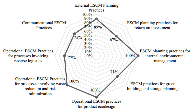
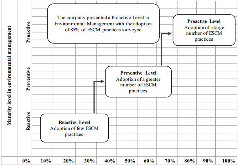
This research aimed to identify the level of maturity in environmental management in a focal company of a pulp and paper supply chain. Methodologically, it is characterized as a qualitative exploratory case study. Semi-structured interviews were used to collect the data. The adoption and use of Environmental Management Supply Chain (ESCM) practices was assessed using a model based on 53 practices grouped into 8 types of practices. Qualitative data analysis software (NVivo) was used to analyse the data and support the development of findings. It was found that 85% of the ESCM practices were adopted by the company. Internal environmental management practices, waste and risk minimization and eco-design were fully adopted. Furthermore, a proactive maturity level was found, embedded in the company's strategic planning. Proactivity in environmental management encourages continuous improvement, cost reduction, cleaner production, and reuse and recycling of products.
Citation: Antonio Zanin, Ivonez Xavier de Almeida, Francieli Pacassa, Fabricia Silva da Rosa, Paulo Afonso. Maturity level of environmental management in the pulp and paper supply chain[J]. AIMS Environmental Science, 2021, 8(6): 580-596. doi: 10.3934/environsci.2021037
This research aimed to identify the level of maturity in environmental management in a focal company of a pulp and paper supply chain. Methodologically, it is characterized as a qualitative exploratory case study. Semi-structured interviews were used to collect the data. The adoption and use of Environmental Management Supply Chain (ESCM) practices was assessed using a model based on 53 practices grouped into 8 types of practices. Qualitative data analysis software (NVivo) was used to analyse the data and support the development of findings. It was found that 85% of the ESCM practices were adopted by the company. Internal environmental management practices, waste and risk minimization and eco-design were fully adopted. Furthermore, a proactive maturity level was found, embedded in the company's strategic planning. Proactivity in environmental management encourages continuous improvement, cost reduction, cleaner production, and reuse and recycling of products.

| [1] |
Ferreira MA, Jabbour CJC, Jabbour ABLS (2017) Maturity levels of material cycles and waste management in a context of green supply chain management: An innovative framework and its application to Brazilian cases. J Mater Cycles Waste 19: 516-525. doi: 10.1007/s10163-015-0416-5

|
| [2] |
Potrich L, Cortimiglia MN, Medeiros JF (2019) A systematic literature review on firm-level proactive environmental management. J Environ Manage 243: 273-286. doi: 10.1016/j.jenvman.2019.04.110
|
| [3] |
Koberg E, Longoni A (2019) A systematic review of sustainable supply chain management in global supply chains. J Clean Prod 207: 1084-1098. doi: 10.1016/j.jclepro.2018.10.033
|
| [4] |
Green KW, Zelbst PJ, Meacham J, et al. (2012) Green supply chain management practices: impact on performance. Supply Chain Manag 17: 290-305. doi: 10.1108/13598541211227126
|
| [5] | Zhu Q, Sarkis J, Lai K (2007) Green supply chain management: pressures, practices and performance within the Chinese automobile industry. J Clean Prod 15: 11-12, 1041-1052. |
| [6] |
Sharma VK, Chandna P, Bhardwaj A (2017) Green supply chain management related performance indicators in agro industry: A review. J Clean Prod 141: 1194-1208. doi: 10.1016/j.jclepro.2016.09.103
|
| [7] |
Shultz CJ, Holbrook MB (1999) Marketing and the tragedy of the commons: A synthesis, commentary, and analysis for action. J Public Policy Mar 18: 218-229. doi: 10.1177/074391569901800208
|
| [8] |
Rao P, Holt D (2005) Do green supply chains lead to competitiveness and economic performance? Int J Oper Prod Man 25: 898-916. doi: 10.1108/01443570510613956
|
| [9] | Jain VK, Sharma S (2014) Drivers Affecting the Green Supply Chain Management Adaptation: A Review. IUP J Oper Manag 13: 54-63. |
| [10] |
Camargo TF, Zanin A, Mazzioni S, et al. (2018) Sustainability indicators in the swine industry of the Brazilian State of Santa Catarina. Environ Dev Sustain 20: 65-81. doi: 10.1007/s10668-018-0147-6
|
| [11] |
Srivastava SK (2007) Green supply-chain management: a state-of-the-art literature review. Int J Manag Rev 9: 53-80. doi: 10.1111/j.1468-2370.2007.00202.x
|
| [12] |
Darnall N, Jolley GJ, Handfield R (2008) Environmental management systems and green supply chain management: complements for sustainability? Bus Strat Environ 17: 30-45. doi: 10.1002/bse.557
|
| [13] |
Wu GC, Ding JH, Chen PS (2012) The effects of GSCM drivers and institutional pressures on GSCM practices in Taiwan's textile and apparel industry. Int J Prod Econ 135: 618-636. doi: 10.1016/j.ijpe.2011.05.023
|
| [14] |
Jabbour ABLS, Jabbour CJC, Latan H, et al (2014) Quality management, environmental management maturity, green supply chain practices and green performance of Brazilian companies with ISO 14001 certification: Direct and indirect effects. Transport Research E-Log 67: 39-51. doi: 10.1016/j.tre.2014.03.005
|
| [15] |
Maialle G, Jabbour ABLS, Arantes AF, et al. (2016) Environmental management maturity of local and multinational high-technology corporations located in Brazil: the role of business internationalization in pollution prevention. Production 26: 488-499. doi: 10.1590/0103-6513.176914
|
| [16] | Ferreira MA, Jabbour CJC (2019) Relating maturity levels in environmental management by adopting Green Supply Chain Management practices: Theoretical convergence and multiple case study. Gestão e Produção 26: 1-17. |
| [17] |
Gunarathne N, Lee KH (2019) Institutional pressures and corporate environmental management maturity. Manag Environ Qual: An Int J 30: 157-175. doi: 10.1108/MEQ-02-2018-0041
|
| [18] |
Ormazabal M, Sarriegi JM, Rich E, et al. (2020) Environmental Management Maturity: The Role of Dynamic Validation. Organ Environ 34: 145-170. doi: 10.1177/1086026620929058
|
| [19] |
Pimenta HCD, Ball PD (2015) Analysis of environmental sustainability practices across upstream supply chain management. Procedia Cirp 26: 677-682. doi: 10.1016/j.procir.2014.07.036
|
| [20] | Costa Filho BA, Rosa F (2017) Maturidade em gestão ambiental: Revisitando as melhores práticas. Revista Eletrônica de Administração: 23: 110-134. |
| [21] | Jabbour CJC, Santos FCA, Nagano MS (2009) Análise do relacionamento entre estágios evolutivos da gestão ambiental e dimensões de recursos humanos: estado da arte e survey em empresas brasileiras. Revista de Administração-RAUSP 44: 342-364. |
| [22] | Zanin A, Dal Magro CB, Mazzioni S, et al. (2019) Triple Bottom Line Analysis in an Agribusiness Supply Chain. International Joint Conference on Industrial Engineering and Operations Management 264-273. |
| [23] |
Zanin A, Dal Magro CB, Kleinibing Bugalho D, et al. (2020) Driving Sustainability in Dairy Farming from a TBL Perspective: Insights from a Case Study in the West Region of Santa Catarina, Brazil. Sustainability 12: 6038-6056. doi: 10.3390/su12156038
|
| [24] | Jabbour CJC (2007) Contribuições da gestão de recursos humanos para a evolução da gestão ambiental empresarial: survey e estudo de múltiplos casos. Universidade de São Paulo. |
| [25] |
Sheu JB, Chou YH, Hu CC (2005) An integrated logistics operational model for green-supply chain management. Transport Research E-Log 41: 287-313. doi: 10.1016/j.tre.2004.07.001
|
| [26] |
Beamon BM (1999) Designing the green supply chain. Logistics Information Management 12: 332-342. doi: 10.1108/09576059910284159
|
| [27] |
Zhu Q, Sarkis J, Geng Y (2005) Green supply chain management in China: pressures, practices and performance. Int J Oper Prod Man 25: 449-468. doi: 10.1108/01443570510593148
|
| [28] | Barve A, Muduli K (2011) Challenges to environmental management practices in Indian mining industries. International Conference on Innovation, Management and Service IPEDR 14: 297-302. |
| [29] |
Sarkis J (2003) A strategic decision framework for green supply chain management. J Clean Prod 11: 397-409. doi: 10.1016/S0959-6526(02)00062-8
|
| [30] |
Zhu Q, Sarkis J (2004) Relationships between operational practices and performance among early adopters of green supply chain management practices in Chinese manufacturing enterprises. J Oper Mana 22: 265-289. doi: 10.1016/j.jom.2004.01.005
|
| [31] | Naslund D, Williamson S (2010) What is management in supply chain management? - a critical review of definitions, frameworks and terminology. J Manag Pol Practice 11: 11-28. |
| [32] |
Gupta V, Abidi N, Bandyopadhayay A (2013) Supply chain management - a three dimensional framework. J Manag Res 5: 76-97. doi: 10.5296/jmr.v5i4.3986
|
| [33] |
Vachon S, Klassen R D (2008) Environmental management and manufacturing performance: The role of collaboration in the supply chain. Int J Prod Econ 111: 299-315. doi: 10.1016/j.ijpe.2006.11.030
|
| [34] |
Eltayeb TK, Zailani S, Ramayah T (2011) Green supply chain initiatives among certified companies in Malaysia and environmental sustainability: Investigating the outcomes. Res Conserv Recy 55: 495-506. doi: 10.1016/j.resconrec.2010.09.003
|
| [35] |
Sulistio J, Rini TA (2015) A structural literature review on models and methods analysis of green supply chain management. Procedia Manuf 4: 291-299. doi: 10.1016/j.promfg.2015.11.043
|
| [36] | Min H, Galle WP (1997) Green purchasing strategies: trends and implications. Int J Purch Mater Manag 33: 10-17. |
| [37] |
Hervani AA, Helms MM, Sarkis J (2005) Performance measurement for green supply chain management. Benchmark: An Int J 12: 330-353. doi: 10.1108/14635770510609015
|
| [38] | Kafa N, Hani Y, El Mhamedi A (2013) Sustainability performance measurement for green supply chain management. IFAC Proceedings 46: 71-78. |
| [39] |
González BJ, González BÓ (2006) A review of determinant factors of environmental proactivity. Bus Strat Environ: 15: 87-102. doi: 10.1002/bse.450
|
| [40] |
Rehman MAA, Shrivastava RL (2011) An innovative approach to evaluate green supply chain management (GSCM) drivers by using interpretive structural modeling (ISM). Int J Innov Technol Manag 8: 315-336. doi: 10.1142/S0219877011002453
|
| [41] |
Chin TA, Tat HH, Sulaiman Z. (2015) Green supply chain management, environmental collaboration and sustainability performance. Procedia Cirp 26: 695-699. doi: 10.1016/j.procir.2014.07.035
|
| [42] |
Liu R, Zhang P, Wang X, et al. (2013) Assessment of effects of best management practices on agricultural non-point source pollution in Xiangxi River watershed. Agr Water Manage 117: 9-18. doi: 10.1016/j.agwat.2012.10.018
|
| [43] |
Jabbour ABLS, Vasquez BD, Jabbour CJC, et al. (2017) Green supply chain practices and environmental performance in Brazil: Survey, case studies, and implications for B2B. Ind Market Manag 66: 13-28. doi: 10.1016/j.indmarman.2017.05.003
|
| [44] | Walton SV, Handfield RB, Melnyk SA (1998) The green supply chain: integrating suppliers into environmental management processes. Int J Purchas Mater Manag 34: 2-11. |
| [45] |
Teixeira AA, Jabbour CJC, Latan H, et al. (2019) The importance of quality management for the effectiveness of environmental management: Evidence from companies located in Brazil. Total Qual Manag Bus 30: 1338-1349. doi: 10.1080/14783363.2017.1368377
|
| [46] |
Azevedo SG, Carvalho H, Machado VC (2011) The influence of green practices on supply chain performance: A case study approach. Transport Research E-Log 47: 850-871. doi: 10.1016/j.tre.2011.05.017
|
| [47] |
Jabbour CJC (2010) Non-linear pathways of corporate environmental management: a survey of ISO 14001-certified companies in Brazil. J Clean Prod 18: 1222-1225. doi: 10.1016/j.jclepro.2010.03.012
|
| [48] |
Jabbour CJC (2015) Environmental training and environmental management maturity of Brazilian companies with ISO14001: empirical evidence. J Clean Prod 96: 331-338. doi: 10.1016/j.jclepro.2013.10.039
|
| [49] | Jabbour CJC, Santos FCA (2006) Evolução da gestão ambiental na empresa: uma taxonomia integrada à gestão da produção e de recursos humanos. Gestão & Produção 13: 435-448. |
| [50] |
Geng R, Mansouri SA, Aktas E (2017) The relationship between green supply chain management and performance: A meta-analysis of empirical evidences in Asian emerging economies. Int J Prod Econ 183: 245-258. doi: 10.1016/j.ijpe.2016.10.008
|
| [51] |
Mitra S, Datta PP (2014) Adoption of green supply chain management practices and their impact on performance: an exploratory study of Indian manufacturing firms. Int J Prod Res 52: 2085-2107. doi: 10.1080/00207543.2013.849014
|
| [52] |
Zhu Q, Sarkis J, Lai K, et al. (2008) The role of organizational size in the adoption of green supply chain management practices in China. Corp Soc Respon Environ Manag 15: 322-337. doi: 10.1002/csr.173
|
| [53] | Ninlawan C, Seksan P, Tossapol K, et al. (2010) The implementation of green supply chain management practices in electronics industry. World Congress on Engineering 2012. July 4-6, 2012. London, UK., 2182, 1563-1568. |
| [54] | Sharma M (2014) The role of employees' engagement in the adoption of green supply chain practices as moderated by environment attitude: An empirical study of the Indian automobile industry. Global Bus Rev 15: 4, 25-38. |
| [55] |
Tate WL, Ellram LM, Kirchoff JF (2010) Corporate social responsibility reports: a thematic analysis related to supply chain management. J Supply Chain Manag 46: 19-44. doi: 10.1111/j.1745-493X.2009.03184.x
|
| [56] | Henriques I, Sadorsky P (1999) The relationship between environmental commitment and managerial perceptions of stakeholder importance. Academy of Management Journal 42: 87-99. |
| [57] |
Seuring S, Müller M (2008) From a literature review to a conceptual framework for sustainable supply chain management. J Clean Prod 16: 1699-1710. doi: 10.1016/j.jclepro.2008.04.020
|
| [58] |
Kuei C, Madu CN, Chow WS, et al. (2015) Determinants and associated performance improvement of green supply chain management in China. J Clean Prod: 95,163-173. doi: 10.1016/j.jclepro.2015.02.030
|
| [59] |
Masoumik SM, Abdul-Rashid SH, Olugu EU, et al. (2015) A strategic approach to develop green supply chains. Procedia Cirp 26: 670-676. doi: 10.1016/j.procir.2014.07.091
|
| [60] |
DiMaggio PJ, Powell WW (1983) The iron cage revisited: Institutional isomorphism and collective rationality in organizational fields. Am Sociol Rev 48: 147-160. doi: 10.2307/2095101
|
| [61] |
Meyer JW, Rowan B (1977) Institutionalized organizations: Formal structure as myth and ceremony. Am J Sociol 83: 340-363. doi: 10.1086/226550
|
| [62] |
Alvesson M, Spicer A (2019) Neo-institutional theory and organization studies: a mid-life crisis? Organ Stud 40: 199-218. doi: 10.1177/0170840618772610
|
| [63] | Guerreiro R, Frezatti F, Lopes AB, et al. (2005) O entendimento da contabilidade gerencial sob a ótica da teoria institucional. Organizações & Sociedade 12: 91-106. |
| [64] | Cunha PR, Santos V, Beuren IM (2015) Artigos de periódicos internacionais que relacionam teoria institucional com contabilidade gerencial. Perspectivas Contemporâneas 10: 1-23. |
| [65] |
Machado da Silva CL, Fonseca VS, Crubellate JM (2005) Estrutura, agência e interpretação: elementos para uma abordagem recursiva do processo de institucionalização. RAC-Revista de Administração Contemporânea 9: 9-39. doi: 10.1590/S1415-65552005000500002
|
| [66] |
Sarkis J, Zhu Q, Lai K (2011) An organizational theoretic review of green supply chain management literature. Int J Prod Econ 130: 1-15. doi: 10.1016/j.ijpe.2010.11.010
|
| [67] |
Zhu Q, Sarkis J, Lai K (2013) Institutional-based antecedents and performance outcomes of internal and external green supply chain management practices. J Purchas Supply Manag 19: 106-117. doi: 10.1016/j.pursup.2012.12.001
|
| [68] |
Geffen CA, Rothenberg S (2000) Suppliers and environmental innovation. Int J Oper Prod Man 20: 166-186. doi: 10.1108/01443570010304242
|
| [69] |
Zhu Q, Sarkis J, Lai K (2012) Green supply chain management innovation diffusion and its relationship to organizational improvement: An ecological modernization perspective. J Eng Technol Manage 29: 168-185. doi: 10.1016/j.jengtecman.2011.09.012
|
| [70] |
Nikolopoulou A, Ierapetritou MG (2012) Optimal design of sustainable chemical processes and supply chains: A review. Comput Chem Eng 44: 94-103. doi: 10.1016/j.compchemeng.2012.05.006
|
| [71] | Corazza RI (2003) Gestão ambiental e mudanças da estrutura organizacional. RAE Eletrônica 2: 1-23 |
Figures(2) / Tables(1)

Antonio Zanin, Ivonez Xavier de Almeida, Francieli Pacassa, Fabricia Silva da Rosa, Paulo Afonso. Maturity level of environmental management in the pulp and paper supply chain[J]. AIMS Environmental Science, 2021, 8(6): 580-596. doi: 10.3934/environsci.2021037


 DownLoad: