Dementia is a prevalent, progressive, neurodegenerative condition with multifactorial causes. Due to the lack of effective pharmaceutical treatments for dementia, there are growing clinical and research interests in using vagus nerve stimulation (VNS) as a potential non-pharmacological therapy for dementia. However, the extent of the research volume and nature into the effects of VNS on dementia is not well understood. This study aimed to examine the extent and nature of research activities in relation to the use of VNS in dementia and disseminate research findings for the potential utility in dementia care.
We performed a scoping review of literature searches in PubMed, HINARI, Google Scholar, and the Cochrane databases from 1980 to November 30th, 2023, including the reference lists of the identified studies. The following search terms were utilized: brain stimulation, dementia, Alzheimer's disease, vagal stimulation, memory loss, Deme*, cognit*, VNS, and Cranial nerve stimulation. The included studies met the following conditions: primary research articles pertaining to both humans and animals for both longitudinal and cross-sectional study designs and published in English from January 1st, 1980, to November 30th, 2023; investigated VNS in either dementia or cognitive impairment; and were not case studies, conference proceedings/abstracts, commentaries, or ordinary review papers.
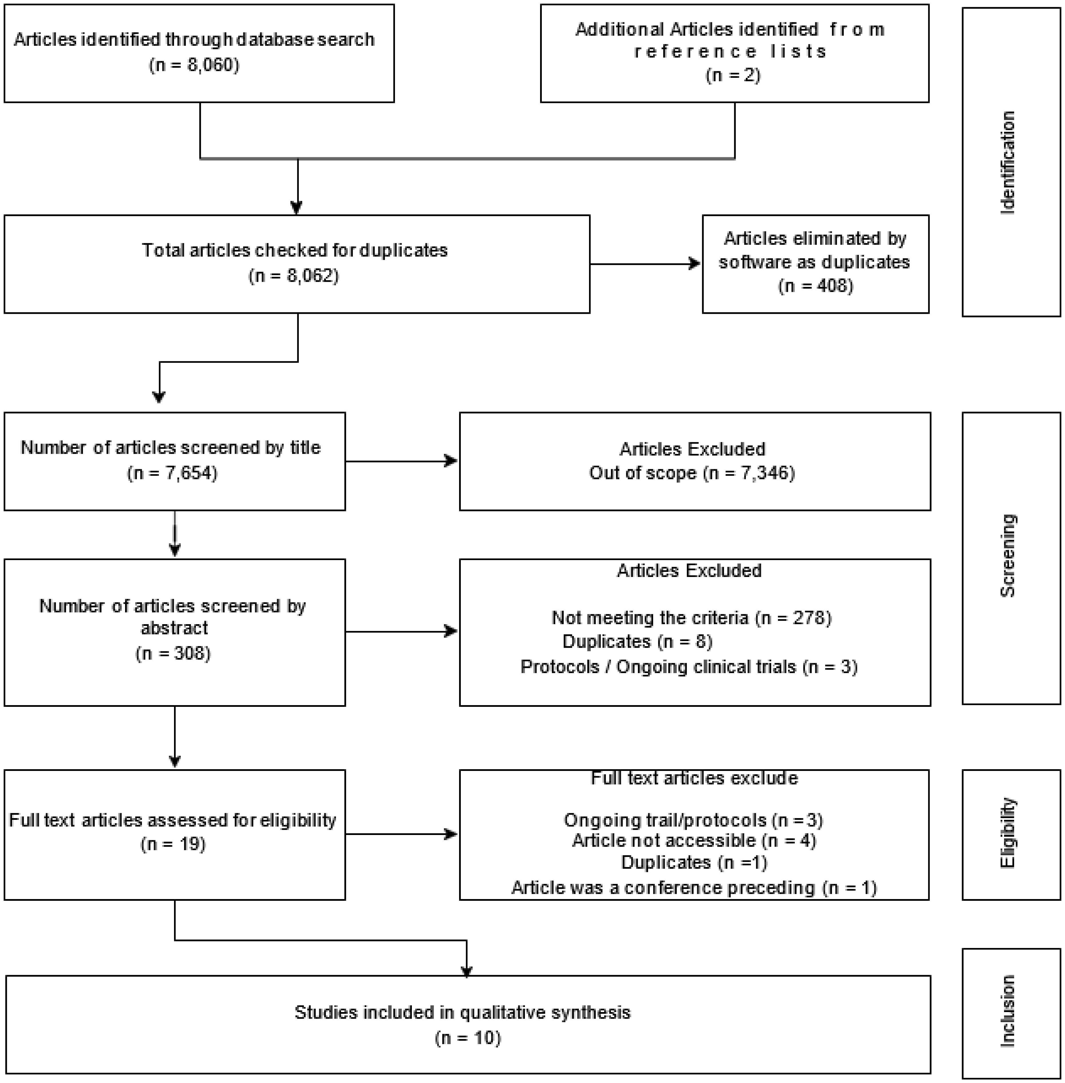
We identified 8062 articles, and after screening for eligibility (sequentially by titles, abstracts and full text reading, and duplicate removal), 10 studies were included in the review. All the studies included in this literature review were conducted over the last three decades in high-income geographical regions (i.e., Europe, the United States, the United Kingdom, and China), with the majority of them (7/10) being performed in humans. The main reported outcomes of VNS in the dementia cases were enhanced cognitive functions, an increased functional connectivity of various brain regions involved in learning and memory, microglial structural modifications from neurodestructive to neuroprotective configurations, a reduction of cerebral spinal fluid tau-proteins, and significant evoked brain tissue potentials that could be utilized to diagnose neurodegenerative disorders. The study outcomes highlight the potential for VNS to be used as a non-pharmacological therapy for cognitive impairment in dementia-related diseases such as Alzheimer's disease.
Citation: Ronald Kamoga, Godfrey Zari Rukundo, Samuel Kalungi, Wilson Adriko, Gladys Nakidde, Celestino Obua, Johnes Obongoloch, Amadi Ogonda Ihunwo. Vagus nerve stimulation in dementia: A scoping review of clinical and pre-clinical studies[J]. AIMS Neuroscience, 2024, 11(3): 398-420. doi: 10.3934/Neuroscience.2024024
Dementia is a prevalent, progressive, neurodegenerative condition with multifactorial causes. Due to the lack of effective pharmaceutical treatments for dementia, there are growing clinical and research interests in using vagus nerve stimulation (VNS) as a potential non-pharmacological therapy for dementia. However, the extent of the research volume and nature into the effects of VNS on dementia is not well understood. This study aimed to examine the extent and nature of research activities in relation to the use of VNS in dementia and disseminate research findings for the potential utility in dementia care.
We performed a scoping review of literature searches in PubMed, HINARI, Google Scholar, and the Cochrane databases from 1980 to November 30th, 2023, including the reference lists of the identified studies. The following search terms were utilized: brain stimulation, dementia, Alzheimer's disease, vagal stimulation, memory loss, Deme*, cognit*, VNS, and Cranial nerve stimulation. The included studies met the following conditions: primary research articles pertaining to both humans and animals for both longitudinal and cross-sectional study designs and published in English from January 1st, 1980, to November 30th, 2023; investigated VNS in either dementia or cognitive impairment; and were not case studies, conference proceedings/abstracts, commentaries, or ordinary review papers.
We identified 8062 articles, and after screening for eligibility (sequentially by titles, abstracts and full text reading, and duplicate removal), 10 studies were included in the review. All the studies included in this literature review were conducted over the last three decades in high-income geographical regions (i.e., Europe, the United States, the United Kingdom, and China), with the majority of them (7/10) being performed in humans. The main reported outcomes of VNS in the dementia cases were enhanced cognitive functions, an increased functional connectivity of various brain regions involved in learning and memory, microglial structural modifications from neurodestructive to neuroprotective configurations, a reduction of cerebral spinal fluid tau-proteins, and significant evoked brain tissue potentials that could be utilized to diagnose neurodegenerative disorders. The study outcomes highlight the potential for VNS to be used as a non-pharmacological therapy for cognitive impairment in dementia-related diseases such as Alzheimer's disease.

| [1] | WHOGlobal action plan on the public health response to Dementia 2017-2025. In (2023). |
| [2] |
Von Ah D, Jansen CE, Allen D, et al. (2011) Putting evidence into practice: evidence-based interventions for cancer and cancer treatment-related cognitive impairment. Clin J Oncol Nurs 15: 607-615. https://doi.org/10.1188/11.CJON.607-615 
|
| [3] |
Metin B, Krebs RM, Wiersema JR, et al. (2015) Dysfunctional modulation of default mode network activity in attention-deficit/hyperactivity disorder. J Abnorm Psychol 124: 208-214. https://doi.org/10.1037/abn0000013
|
| [4] | Wolf A, Bauer B, Abner EL, et al. (2016) A comprehensive behavioral test battery to assess learning and memory in 129S6/Tg2576 mice. PloS One 11. https://doi.org/10.1371/journal.pone.0147733 |
| [5] |
Shafqat S (2008) Alzheimer disease therapeutics: perspectives from the developing world. J Alzheimers Dis 15: 285-287. https://doi.org/10.3233/JAD-2008-15211
|
| [6] |
Chang CH, Lane HY, Lin CH (2018) Brain stimulation in Alzheimer's disease. Front Psychiatry 9: 201. https://doi.org/10.3389/fpsyt.2018.00201
|
| [7] |
Conway CR, Kumar A, Xiong W, et al. (2018) Chronic vagus nerve stimulation significantly improves quality of life in treatment-resistant major depression. J Clin Psychiatry 79: 22269. https://doi.org/10.4088/JCP.18m12178
|
| [8] |
De Ferrari GM, Schwartz PJ (2011) Vagus nerve stimulation: from pre-clinical to clinical application: challenges and future directions. Heart Fail Rev 16: 195-203. https://doi.org/10.1007/s10741-010-9216-0
|
| [9] |
Kumar A, Bunker MT, Aaronson ST, et al. (2019) Durability of symptomatic responses obtained with adjunctive vagus nerve stimulation in treatment-resistant depression. Neuropsych Dis Treat : 457-468. https://doi.org/10.2147/NDT.S196665
|
| [10] |
Ruffoli R, Giorgi FS, Pizzanelli C, et al. (2011) The chemical neuroanatomy of vagus nerve stimulation. J Chem Neuroanat 42: 288-296. https://doi.org/10.1016/j.jchemneu.2010.12.002
|
| [11] |
Engineer ND, Kimberley TJ, Prudente CN, et al. (2015) Targeted Vagus Nerve Stimulation for Rehabilitation After Stroke. Front Neurosci 13: 280. https://doi.org/10.3389/fnins.2019.00280
|
| [12] |
Friedman NI (2016) Brain Stimulation in Alzheimer's disease. J Alzheimers Dis 54: 789-791. https://doi.org/10.3233/JAD-160719
|
| [13] |
Ma X, Wang Q, Ong JJ, et al. (2018) Prevalence of human papillomavirus by geographical regions, sexual orientation and HIV status in China: a systematic review and meta-analysis. Sex Transm Infect 94: 434-442. https://doi.org/10.1136/sextrans-2017-053412
|
| [14] |
Pesavento E, Capsoni S, Domenici L, et al. (2002) Acute cholinergic rescue of synaptic plasticity in the neurodegenerating cortex of anti-nerve-growth-factor mice. Eur J Neurosci 15: 1030-1036. https://doi.org/10.1046/j.1460-9568.2002.01937.x
|
| [15] |
Ansari S, Chaudhri K, Moutaery KA (2007) Vagus nerve stimulation: indications and limitations. Acta Neurochir Suppl 97: 281-286. https://doi.org/10.1007/978-3-211-33081-4_31
|
| [16] |
Ghacibeh GA, Shenker JI, Shenal B, et al. (2006) The influence of vagus nerve stimulation on memory. Cogn Behav Neurol 19: 119-122. https://doi.org/10.1097/01.wnn.0000213908.34278.7d
|
| [17] |
Kosel M, Schlaepfer TE (2003) Beyond the treatment of epilepsy: new applications of vagus nerve stimulation in psychiatry. CNS Spectrums 8: 515-521. https://doi.org/10.1017/S1092852900018988
|
| [18] |
Merrill CA, Jonsson MAG, Minthon L, et al. (2006) Vagus nerve stimulation in patients with Alzheimer's disease: additional follow-up results of a pilot study through 1 year. J Clin Psychiatry 67: 1171-1178. https://doi.org/10.4088/JCP.v67n0801
|
| [19] |
Roy DS, Arons A, Mitchell TI, et al. (2016) Memory retrieval by activating engram cells in mouse models of early Alzheimer's disease. Nature 531: 508-512. https://doi.org/10.1038/nature17172
|
| [20] |
Sun Q, Xie N, Tang B, et al. (2017) Alzheimer's disease: from genetic variants to the distinct pathological mechanisms. Front Mol Neurosci 10: 319. https://doi.org/10.3389/fnmol.2017.00319
|
| [21] |
Ghacibeh GA, Shenker JI, Shenal B, et al. (2006) Effect of vagus nerve stimulation on creativity and cognitive flexibility. Epilepsy Behav 8: 720-725. https://doi.org/10.1016/j.yebeh.2006.03.008
|
| [22] |
Tricco AC, Lillie E, Zarin W, et al. (2018) PRISMA extension for scoping reviews (PRISMA-ScR): checklist and explanation. Ann Intern Med 169: 467-473. https://doi.org/10.7326/M18-0850
|
| [23] |
Moher D, Liberati A, Tetzlaff J, et al. (2009) Preferred reporting items for systematic reviews and meta-analyses: the PRISMA statement. Ann Intern Med 151: 264-269. https://doi.org/10.7326/0003-4819-151-4-200908180-00135
|
| [24] |
Broncel A, Bocian R, Kłos-Wojtczak P, et al. (2020) Vagal nerve stimulation as a promising tool in the improvement of cognitive disorders. Brain Res Bull 155: 37-47. https://doi.org/10.1016/j.brainresbull.2019.11.011
|
| [25] |
Vargas-Caballero M, Warming H, Walker R, et al. (2022) Vagus nerve stimulation as a potential therapy in early Alzheimer's disease: A review. Front Hum Neurosci 16: 866434. https://doi.org/10.3389/fnhum.2022.866434
|
| [26] |
Moher D, Liberati A, Tetzlaff J, et al. (2009) Preferred reporting items for systematic reviews and meta-analyses: the PRISMA statement. Ann Intern Med 151: 264-269. https://doi.org/10.7326/0003-4819-151-4-200908180-00135
|
| [27] | Peters MD, Godfrey CM, Khalil H, et al. (2015) Guidance for conducting systematic scoping reviews. JBI Evid Implement 13: 141-146. https://doi.org/10.1097/XEB.0000000000000050 |
| [28] | MDJ P, GC M: Scoping Review. Joanna Briggs Institute Reviewer's Manual (2017) . |
| [29] | Wang L, Zhang J, Lu X, et al. The Mechanism Underlying Chronic Transcutaneous Auricular Vagus Nerve Stimulation in Patients with Mild Cognitive Impairment Through the Enhancement of the Functional Connectivity between the Left Precuneus and Parahippocampus Gyrus (2023). Available from: https://doi.org/10.2139/ssrn.4369340 |
| [30] |
Wang L, Zhang J, Guo C, et al. (2022) The efficacy and safety of transcutaneous auricular vagus nerve stimulation in patients with mild cognitive impairment: a double blinded randomized clinical trial. Brain Stimul 15: 1405-1414. https://doi.org/10.1016/j.brs.2022.09.003
|
| [31] |
Metzger FG, Polak T, Aghazadeh Y, et al. (2012) Vagus somatosensory evoked potentials--a possibility for diagnostic improvement in patients with mild cognitive impairment?. Dement Geriatr Cogn Disord 33: 289-296. https://doi.org/10.1159/000339359
|
| [32] |
Murphy AJ, O'Neal AG, Cohen RA, et al. (2023) The Effects of Transcutaneous Vagus Nerve Stimulation on Functional Connectivity Within Semantic and Hippocampal Networks in Mild Cognitive Impairment. Neurotherapeutics 20: 419-430. https://doi.org/10.1007/s13311-022-01318-4
|
| [33] |
Merrill CA, Bunker M (2004) P3-032 Effects of vagus nerve stimulation on cognition, CSF-Tau and cerebral blood flow in patients with Alzheimer's disease: results of a 1 year pilot study. Neurobiol Aging 25: S360. https://doi.org/10.1016/S0197-4580(04)81186-2
|
| [34] |
Kaczmarczyk R, Tejera D, Simon BJ, et al. (2018) Microglia modulation through external vagus nerve stimulation in a murine model of Alzheimer's disease. J Neurochem 146: 76-85. https://doi.org/10.1111/jnc.14284
|
| [35] |
Smith DC, Modglin AA, Roosevelt RW, et al. (2005) Electrical stimulation of the vagus nerve enhances cognitive and motor recovery following moderate fluid percussion injury in the rat. J Neurotraum 22: 1485-1502. https://doi.org/10.1089/neu.2005.22.1485
|
| [36] |
Dolphin H, Dyer A, Commins S, et al. (2023) 264 Improvements in associative memory and spatial navigation with acute transcutaneous Vagus Nerve Stimulation in Mild Cognitive Impairment: preliminary data. Age Ageing 52: afad156. 032. https://doi.org/10.1093/ageing/afad156.032
|
| [37] |
O'Neal AG, Cohen R, Porges EC, et al. (2023) 43 Transcutaneous Vagus Nerve Stimulation Effects on Functional Connectivity of the Hippocampus in Mild Cognitive Impairment. J Int Neuropsych Soc 29: 454-454. https://doi.org/10.1017/S1355617723005933
|
| [38] |
Clark KB, Naritoku DK, Smith DC, et al. (1999) Enhanced recognition memory following vagus nerve stimulation in human subjects. Nat Neurosci 2: 94-98. https://doi.org/10.1038/4600
|
| [39] |
Merrill CA, Jonsson MA, Minthon L, et al. (2006) Vagus nerve stimulation in patients with Alzheimer's disease: additional follow-up results of a pilot study through 1 year. J Clin Psychiatry 67: 1171-1178. https://doi.org/10.4088/JCP.v67n0801
|
| [40] |
Sjogren MJ, Hellstrom PT, Jonsson MA, et al. (2002) Cognition-enhancing effect of vagus nerve stimulation in patients with Alzheimer's disease: a pilot study. J Clin Psychiatry 63: 972-980. https://doi.org/10.4088/JCP.v63n1103
|
| [41] |
Kaczmarczyk R, Tejera D, Simon BJ, et al. (2018) Microglia modulation through external vagus nerve stimulation in a murine model of Alzheimer's disease. J Neurochem 146: 76-85. https://doi.org/10.1111/jnc.14284
|
| [42] |
Metzger FG, Polak T, Aghazadeh Y, et al. (2012) Vagus Somatosensory Evoked Potentials–A Possibility for Diagnostic Improvement in Patients with Mild Cognitive Impairment?. Dement Geriatr Cogn 33: 289-296. https://doi.org/10.1159/000339359
|
| [43] |
Murphy AJ, O'Neal AG, Cohen RA, et al. (2023) The effects of transcutaneous vagus nerve stimulation on functional connectivity within semantic and hippocampal networks in mild cognitive impairment. Neurotherapeutics 20: 419-430. https://doi.org/10.1007/s13311-022-01318-4
|
| [44] |
Mattap SM, Mohan D, McGrattan AM, et al. (2022) The economic burden of dementia in low-and middle-income countries (LMICs): a systematic review. BMJ Glob Health 7: e007409. https://doi.org/10.1136/bmjgh-2021-007409
|
| [45] |
Schaller S, Mauskopf J, Kriza C, et al. (2015) The main cost drivers in dementia: a systematic review. IntJ Geriatr Psych 30: 111-129. https://doi.org/10.1002/gps.4198
|
| [46] |
Hojman DA, Duarte F, Ruiz-Tagle J, et al. (2017) The cost of dementia in an unequal country: the case of Chile. PLoS One 12: e0172204. https://doi.org/10.1371/journal.pone.0172204
|
| [47] | Hopkins S (2010) Health expenditure comparisons: low, middle and high income countries. Open Health Serv Policy J 3: 21-27. |
| [48] |
Kamoga R, Rukundo GZ, Wakida EK, et al. (2019) Dementia assessment and diagnostic practices of healthcare workers in rural southwestern Uganda: a cross-sectional qualitative study. BMC Health Serv Res 19. https://doi.org/10.1186/s12913-019-4850-2
|
| [49] | Chamma E, Daradich A, Côté D, et al. (2014) Intravital Microscopy, Pathobiology of Human Disease. Academic Press : 3959-3972. https://doi.org/10.1016/B978-0-12-386456-7.07607-3 |
| [50] |
Johnson RL, Wilson CG (2018) A review of vagus nerve stimulation as a therapeutic intervention. J Inflamm Res 11: 203-213. https://doi.org/10.2147/JIR.S163248
|
| [51] |
Braak H, Del Tredici K (2015) The preclinical phase of the pathological process underlying sporadic Alzheimer's disease. Brain 138: 2814-2833. https://doi.org/10.1093/brain/awv236
|
| [52] |
Luo T, Wang Y, Lu G, et al. (2022) Vagus nerve stimulation for super-refractory status epilepticus in febrile infection-related epilepsy syndrome: a pediatric case report and literature review. Childs Nerv Syst 38: 1401-1404. https://doi.org/10.1007/s00381-021-05410-6
|
| [53] |
Révész D, Rydenhag B, Ben-Menachem E (2016) Complications and safety of vagus nerve stimulation: 25 years of experience at a single center. J Neurosurg Pediatr 18: 97-104. https://doi.org/10.3171/2016.1.PEDS15534
|
| [54] |
Smucny J, Visani A, Tregellas JR (2015) Could vagus nerve stimulation target hippocampal hyperactivity to improve cognition in schizophrenia?. Front Psychiatry 6: 135146. https://doi.org/10.3389/fpsyt.2015.00043
|
| [55] |
Carreno FR, Frazer A (2017) Vagal Nerve Stimulation for Treatment-Resistant Depression. Neurotherapeutics 14: 716-727. https://doi.org/10.1007/s13311-017-0537-8
|
| [56] |
Hamilton P, Soryal I, Dhahri P, et al. (2018) Clinical outcomes of VNS therapy with AspireSR(®) (including cardiac-based seizure detection) at a large complex epilepsy and surgery centre. Seizure 58: 120-126. https://doi.org/10.1016/j.seizure.2018.03.022
|
| [57] |
Yap JYY, Keatch C, Lambert E, et al. (2020) Critical Review of Transcutaneous Vagus Nerve Stimulation: Challenges for Translation to Clinical Practice. Front Neurosci 14: 284. https://doi.org/10.3389/fnins.2020.00284
|
| [58] |
Stefan H, Kreiselmeyer G, Kerling F, et al. (2012) Transcutaneous vagus nerve stimulation (t-VNS) in pharmacoresistant epilepsies: a proof of concept trial. Epilepsia 53: e115-118. https://doi.org/10.1111/j.1528-1167.2012.03492.x
|
| [59] |
Hein E, Nowak M, Kiess O, et al. (2013) Auricular transcutaneous electrical nerve stimulation in depressed patients: a randomized controlled pilot study. J Neural Transm 120: 821-827. https://doi.org/10.1007/s00702-012-0908-6
|
| [60] |
Broncel A, Bocian R, Kłos-Wojtczak P, et al. (2020) Vagal nerve stimulation as a promising tool in the improvement of cognitive disorders. Brain Res Bull 155: 37-47. https://doi.org/10.1016/j.brainresbull.2019.11.011
|
| [61] |
Révész D, Rydenhag B, Ben-Menachem E (2016) Complications and safety of vagus nerve stimulation: 25 years of experience at a single center. J Neurosurg Pediatr 18: 97-104. https://doi.org/10.3171/2016.1.PEDS15534
|
| [62] |
Vonck K, Raedt R, Naulaerts J, et al. (2014) Vagus nerve stimulation... 25 years later! What do we know about the effects on cognition?. Neurosci Biobehav Rev 45: 63-71. https://doi.org/10.1016/j.neubiorev.2014.05.005
|
| [63] |
Metin B, Krebs RM, Wiersema JR, et al. (2015) Dysfunctional modulation of default mode network activity in attention-deficit/hyperactivity disorder. J Abnorm Psychol 124: 208. https://doi.org/10.1037/abn0000013
|
| [64] |
Wolf A, Bauer B, Abner EL, et al. (2016) A comprehensive behavioral test battery to assess learning and memory in 129S6/Tg2576 mice. PloS One 11: e0147733. https://doi.org/10.1371/journal.pone.0147733
|
| [65] |
Butt MF, Albusoda A, Farmer AD, et al. (2020) The anatomical basis for transcutaneous auricular vagus nerve stimulation. J Anat 236: 588-611. https://doi.org/10.1111/joa.13122
|
| [66] | Clancy JA The effects of non-invasive neuromodulation on autonomic nervous system function in humans: University of Leeds (2013). |
| [67] |
Colzato L, Beste C (2020) A literature review on the neurophysiological underpinnings and cognitive effects of transcutaneous vagus nerve stimulation: challenges and future directions. J Neurophysiol 123: 1739-1755. https://doi.org/10.1152/jn.00057.2020
|
| [68] |
Ventura-Bort C, Wirkner J, Wendt J, et al. (2021) Establishment of emotional memories is mediated by vagal nerve activation: evidence from noninvasive taVNS. J Neurosci 41: 7636-7648. https://doi.org/10.1523/JNEUROSCI.2329-20.2021
|
| [69] |
Warren CM, Tona KD, Ouwerkerk L, et al. (2019) The neuromodulatory and hormonal effects of transcutaneous vagus nerve stimulation as evidenced by salivary alpha amylase, salivary cortisol, pupil diameter, and the P3 event-related potential. Brain Stimul 12: 635-642. https://doi.org/10.1016/j.brs.2018.12.224
|
| [70] |
Simmonds L, Lagrata S, Stubberud A, et al. (2023) An open-label observational study and meta-analysis of non-invasive vagus nerve stimulation in medically refractory chronic cluster headache. Front Neurol 14: 100426. https://doi.org/10.3389/fneur.2023.1100426
|
| [71] |
Murray AR, Atkinson L, Mahadi MK, et al. (2016) The strange case of the ear and the heart: The auricular vagus nerve and its influence on cardiac control. Auton Neurosci 199: 48-53. https://doi.org/10.1016/j.autneu.2016.06.004
|
| [72] |
Frangos E, Ellrich J, Komisaruk BR (2015) Non-invasive access to the vagus nerve central projections via electrical stimulation of the external ear: fMRI Evidence in Humans. Brain Stimul 8: 624-636. https://doi.org/10.1016/j.brs.2014.11.018
|
| [73] |
Clancy JA, Mary DA, Witte KK, et al. (2014) Non-invasive vagus nerve stimulation in healthy humans reduces sympathetic nerve activity. Brain Stimul 7: 871-877. https://doi.org/10.1016/j.brs.2014.07.031
|
| [74] |
Wang L, Wang Y, Wang Y, et al. (2022) Transcutaneous auricular vagus nerve stimulators: a review of past, present, and future devices. Expert Rev Med Devic 19: 43-61. https://doi.org/10.1080/17434440.2022.2020095
|
| [75] |
Kaczmarczyk M, Antosik-Wójcińska A, Dominiak M, et al. (2021) Use of transcutaneous auricular vagus nerve stimulation (taVNS) in the treatment of drug-resistant depression - a pilot study, presentation of five clinical cases. Psychiatr Pol 55: 555-564. https://doi.org/10.12740/PP/OnlineFirst/115191
|
| [76] |
Sun L, Peräkylä J, Holm K, et al. (2017) Vagus nerve stimulation improves working memory performance. J Clin Exp Neuropsyc 39: 954-964. https://doi.org/10.1080/13803395.2017.1285869
|
| [77] |
Ghacibeh GA, Shenker JI, Shenal B, et al. (2006) The influence of vagus nerve stimulation on memory. Cogn Behav Neurol 19: 119-122. https://doi.org/10.1097/01.wnn.0000213908.34278.7d
|
| [78] |
Wang C, Wang P, Qi G (2023) A new use of transcutaneous electrical nerve stimulation: Role of bioelectric technology in resistant hypertension. Biomed Rep 18: 1-10. https://doi.org/10.3892/br.2023.1621
|
| [79] |
Jongkees BJ, Immink MA, Finisguerra A, et al. (2018) Transcutaneous vagus nerve stimulation (tVNS) enhances response selection during sequential action. Front Psychol 9: 1159. https://doi.org/10.3389/fpsyg.2018.01159
|
| [80] |
Giraudier M, Ventura-Bort C, Weymar M (2020) Transcutaneous vagus nerve stimulation (tVNS) improves high-confidence recognition memory but not emotional word processing. Front Psychol 11: 1276. https://doi.org/10.3389/fpsyg.2020.01276
|
| [81] |
Clark K, Krahl S, Smith D, et al. (1995) Post-training unilateral vagal stimulation enhances retention performance in the rat. Neurobiol Learn Mem 63: 213-216. https://doi.org/10.1006/nlme.1995.1024
|
| [82] |
Desbeaumes Jodoin V, Richer F, Miron JP, et al. (2018) Long-term Sustained Cognitive Benefits of Vagus Nerve Stimulation in Refractory Depression. J Ect 34: 283-290. https://doi.org/10.1097/YCT.0000000000000502
|
| [83] |
Rosso P, Iannitelli A, Pacitti F, et al. (2020) Vagus nerve stimulation and Neurotrophins: a biological psychiatric perspective. Neurosci Biobehav Rev 113: 338-353. https://doi.org/10.1016/j.neubiorev.2020.03.034
|
| [84] |
Follesa P, Biggio F, Gorini G, et al. (2007) Vagus nerve stimulation increases norepinephrine concentration and the gene expression of BDNF and bFGF in the rat brain. Brain Res 1179: 28-34. https://doi.org/10.1016/j.brainres.2007.08.045
|
| [85] |
Gavrilyuk V, Russo CD, Heneka MT, et al. (2002) Norepinephrine increases IκBα expression in astrocytes. J Biol Chem 277: 29662-29668. https://doi.org/10.1074/jbc.M203256200
|
| [86] |
Korchounov A, Ziemann U (2011) Neuromodulatory neurotransmitters influence LTP-like plasticity in human cortex: a pharmaco-TMS study. Neuropsychopharmacology 36: 1894-1902. https://doi.org/10.1038/npp.2011.75
|
| [87] |
Nagahara AH, Merrill DA, Coppola G, et al. (2009) Neuroprotective effects of brain-derived neurotrophic factor in rodent and primate models of Alzheimer's disease. Nat Med 15: 331-337. https://doi.org/10.1038/nm.1912
|
| [88] |
Heneka MT, Nadrigny F, Regen T, et al. (2010) Locus ceruleus controls Alzheimer's disease pathology by modulating microglial functions through norepinephrine. P Natl Acad Sci 107: 6058-6063. https://doi.org/10.1073/pnas.0909586107
|
| [89] |
Streit WJ, Khoshbouei H, Bechmann I (2020) Dystrophic microglia in late-onset Alzheimer's disease. Glia 68: 845-854. https://doi.org/10.1002/glia.23782
|
| [90] |
Perry VH, Holmes C (2014) Microglial priming in neurodegenerative disease. Nat Rev Neurol 10: 217-224. https://doi.org/10.1038/nrneurol.2014.38
|
| [91] |
Mertens A, Naert L, Miatton M, et al. (2020) Transcutaneous vagus nerve stimulation does not affect verbal memory performance in healthy volunteers. Front Psychol 11: 525888. https://doi.org/10.3389/fpsyg.2020.00551
|
| [92] |
Helmstaedter C, Hoppe C, Elger CE (2001) Memory alterations during acute high-intensity vagus nerve stimulation. Epilepsy Res 47: 37-42. https://doi.org/10.1016/S0920-1211(01)00291-1
|
| [93] |
Klinkenberg S, Aalbers MW, Vles JS, et al. (2012) Vagus nerve stimulation in children with intractable epilepsy: a randomized controlled trial. Dev Med Child Neurol 54: 855-861. https://doi.org/10.1111/j.1469-8749.2012.04305.x
|
| [94] |
McGlone J, Valdivia I, Penner M, et al. (2008) Quality of life and memory after vagus nerve stimulator implantation for epilepsy. Can J Neurol Sci 35: 287-296. https://doi.org/10.1017/S0317167100008854
|
| [95] |
Zuo Y, Smith DC, Jensen RA (2007) Vagus nerve stimulation potentiates hippocampal LTP in freely-moving rats. Physiol Behav 90: 583-589. https://doi.org/10.1016/j.physbeh.2006.11.009
|
| [96] |
Arksey H, O'Malley L (2005) Scoping studies: towards a methodological framework. International Journal of Social Research Methodology 8: 19-32. https://doi.org/10.1080/1364557032000119616
|
| [97] | Mays N, Roberts E, Popay J (2001) Synthesising research evidence. Studying the Organisation and Delivery of Health Services: Research Methods . London: Routledge 188-220. |
Figures(1) / Tables(2)

Ronald Kamoga, Godfrey Zari Rukundo, Samuel Kalungi, Wilson Adriko, Gladys Nakidde, Celestino Obua, Johnes Obongoloch, Amadi Ogonda Ihunwo. Vagus nerve stimulation in dementia: A scoping review of clinical and pre-clinical studies[J]. AIMS Neuroscience, 2024, 11(3): 398-420. doi: 10.3934/Neuroscience.2024024


 DownLoad: