Over decades, sulfur has been employed for treatment of many dermatological diseases, several skin and soft tissue, and Staphylococcus infections. Because of its abuse, resistant bacterial strains have emerged. Nanotechnology has presented a new horizon to overcome abundant problems including drug resistance. Nano-sized sulfur has proven to retain bactericidal activity. Consequently, the specific aims of this study are exclusively directed to produce various sulfur nanoparticles formulations with control of particle size and morphology and investigate the antibacterial activity response specifically classified by the category of responses of different formulations, for the treatment of acne vulgaris resistant to conventional antibiotics. In this study, we produced uncoated sulfur nanoparticles (SNPs), sulfur nano-composite with chitosan (CS-SNPs), and sulfur nanoparticles coated with polyethylene glycol (PEG-SNPs) and evaluate their bactericidal impact against Staphylococcus aureus and Staphylococcus epidermidis isolated from 173 patients clinically diagnosed acne vulgaris. Accompanied with molecular investigations of ermB and mecA resistance genes distribution among the isolates. Sulfur nanoparticles were synthesized using acid precipitation method and were characterized by scanning electron microscope (SEM), transmission electron microscopy (TEM), energy dispersed x-ray spectroscopy (EDX), and Fourier transform infrared spectroscopy (FTIR). Moreover, agar diffusion and broth micro-dilution methods were applied to determine their antibacterial activity and their minimum inhibitory concentration. PCR analysis for virulence factors detection. Results: TEM analysis showed particle size of SNPs (11.7 nm), PEG-SNPs (27 nm) and CS-SNPs (33 nm). Significant antibacterial activity from nanoparticles formulations in 100% dimethyl sulfoxide (DMSO) with inhibition zone 30 mm and MIC at 5.5 µg/mL. Furthermore, the prevalence of mecA gene was the most abundant among the isolates while ermB gene was infrequent. Conclusions: sulfur nanoparticles preparations are an effective treatment for most Staphylococcus bacteria causing acne vulgaris harboring multi-drug resistance virulence factors.
Citation: Noha M. Hashem, Alaa El-Din M.S. Hosny, Ali A. Abdelrahman, Samira Zakeer. Antimicrobial activities encountered by sulfur nanoparticles combating Staphylococcal species harboring sccmecA recovered from acne vulgaris[J]. AIMS Microbiology, 2021, 7(4): 481-498. doi: 10.3934/microbiol.2021029
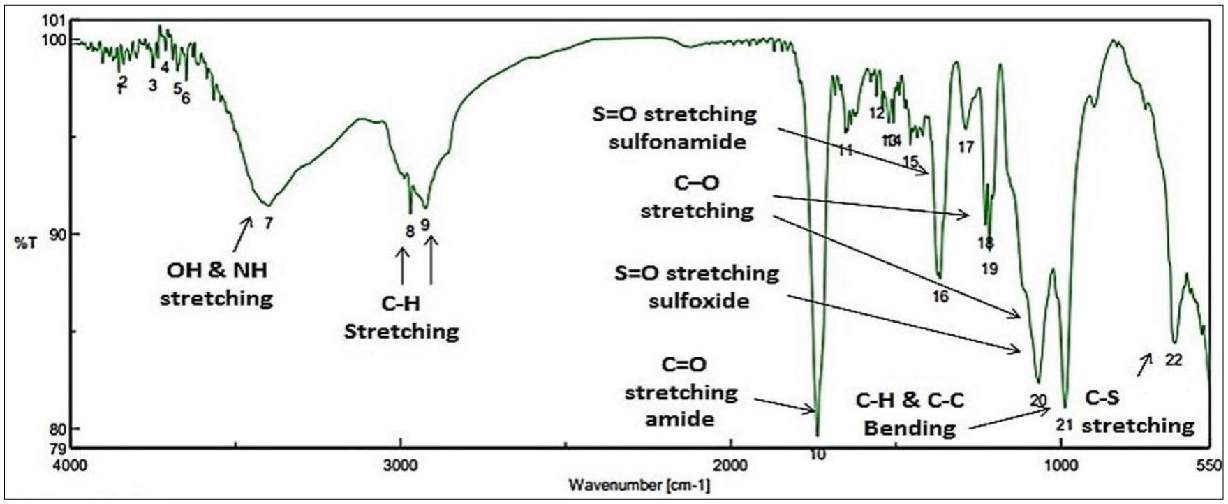
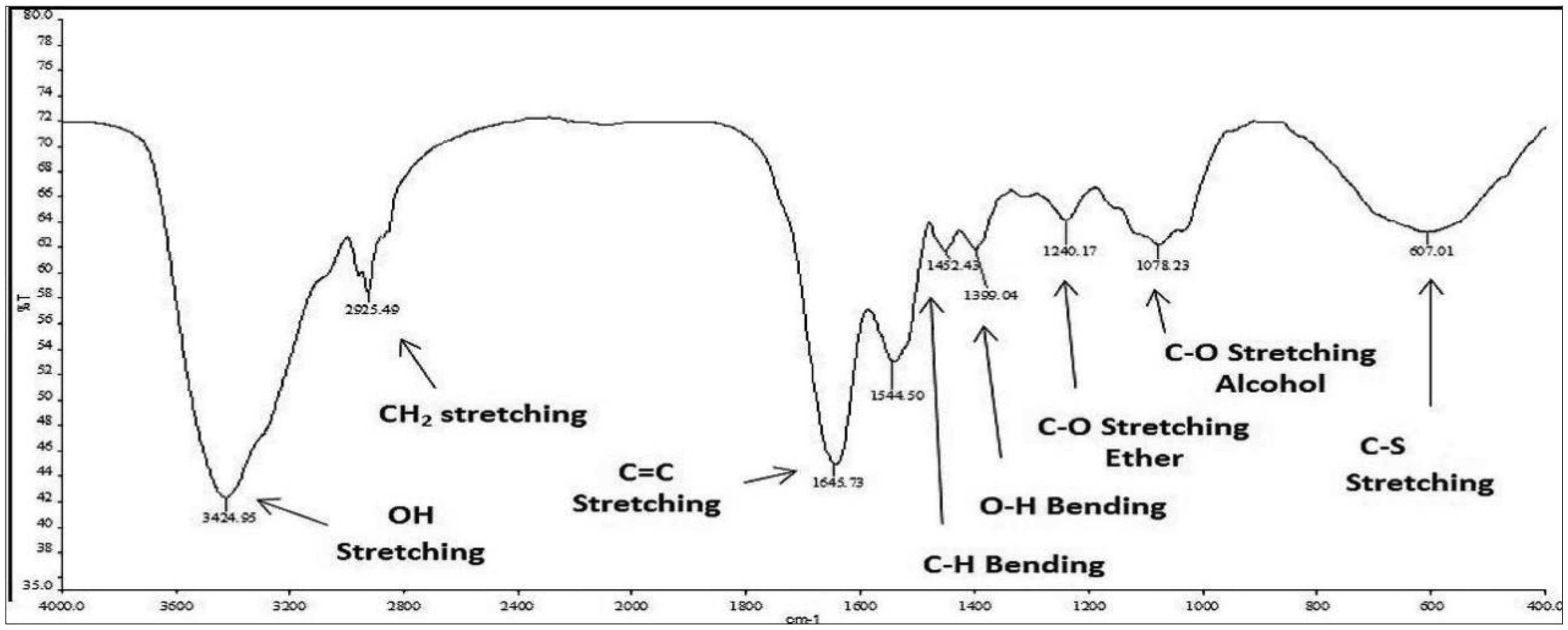
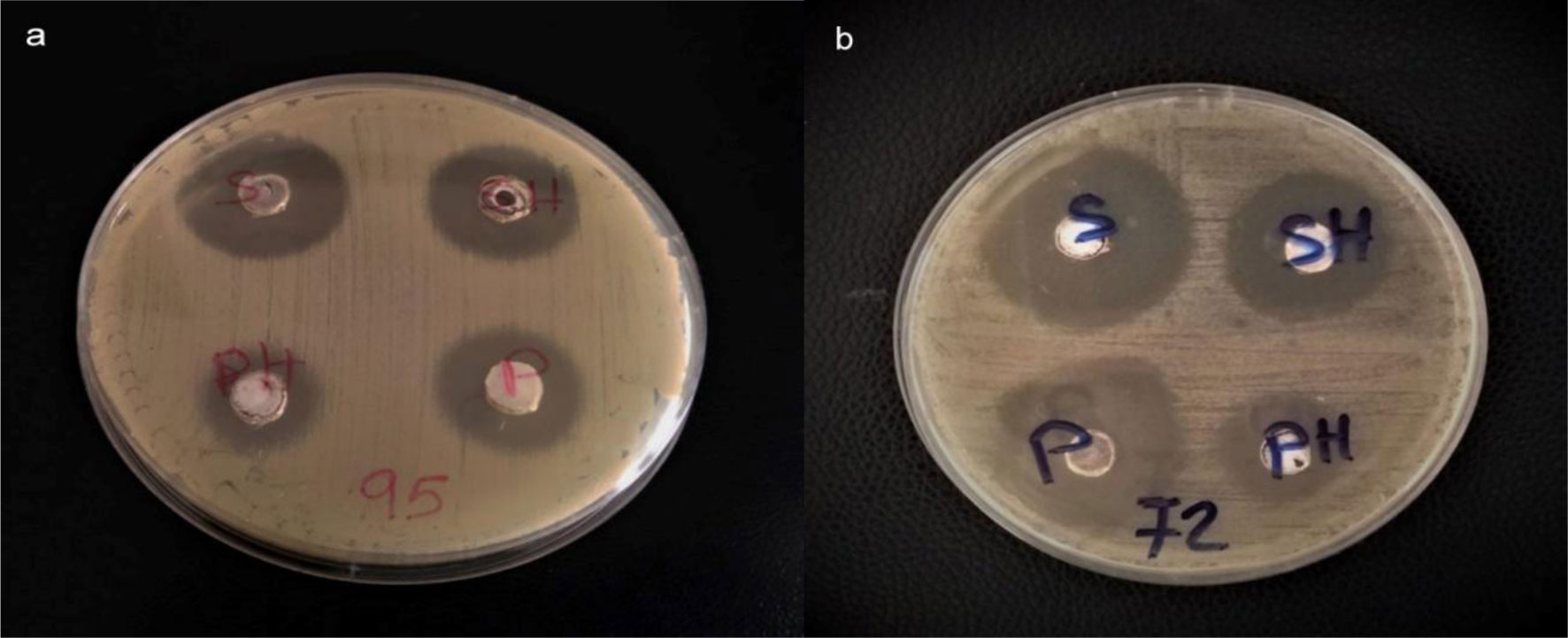
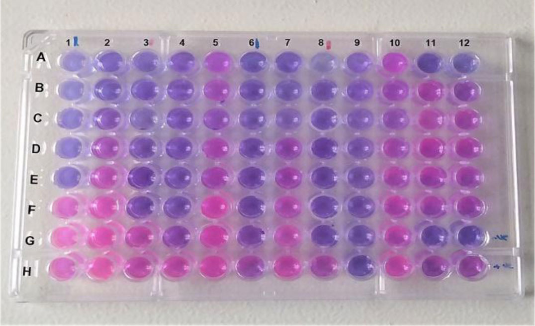
Over decades, sulfur has been employed for treatment of many dermatological diseases, several skin and soft tissue, and Staphylococcus infections. Because of its abuse, resistant bacterial strains have emerged. Nanotechnology has presented a new horizon to overcome abundant problems including drug resistance. Nano-sized sulfur has proven to retain bactericidal activity. Consequently, the specific aims of this study are exclusively directed to produce various sulfur nanoparticles formulations with control of particle size and morphology and investigate the antibacterial activity response specifically classified by the category of responses of different formulations, for the treatment of acne vulgaris resistant to conventional antibiotics. In this study, we produced uncoated sulfur nanoparticles (SNPs), sulfur nano-composite with chitosan (CS-SNPs), and sulfur nanoparticles coated with polyethylene glycol (PEG-SNPs) and evaluate their bactericidal impact against Staphylococcus aureus and Staphylococcus epidermidis isolated from 173 patients clinically diagnosed acne vulgaris. Accompanied with molecular investigations of ermB and mecA resistance genes distribution among the isolates. Sulfur nanoparticles were synthesized using acid precipitation method and were characterized by scanning electron microscope (SEM), transmission electron microscopy (TEM), energy dispersed x-ray spectroscopy (EDX), and Fourier transform infrared spectroscopy (FTIR). Moreover, agar diffusion and broth micro-dilution methods were applied to determine their antibacterial activity and their minimum inhibitory concentration. PCR analysis for virulence factors detection. Results: TEM analysis showed particle size of SNPs (11.7 nm), PEG-SNPs (27 nm) and CS-SNPs (33 nm). Significant antibacterial activity from nanoparticles formulations in 100% dimethyl sulfoxide (DMSO) with inhibition zone 30 mm and MIC at 5.5 µg/mL. Furthermore, the prevalence of mecA gene was the most abundant among the isolates while ermB gene was infrequent. Conclusions: sulfur nanoparticles preparations are an effective treatment for most Staphylococcus bacteria causing acne vulgaris harboring multi-drug resistance virulence factors.

| [1] |
Brook I, Frazier EH, Cox ME, et al. (1995) The aerobic and anaerobic microbiology of pustular acne lesions. Anaerobe 1: 305-307. doi: 10.1006/anae.1995.1031

|
| [2] | Del Rosso JQ, Leyden JJ, Thiboutot D, et al. (2008) Antibiotic use in acne. Cutis 82: 5-12. |
| [3] |
Ito T, Katayama Y, Hiramatsu K (1999) Cloning and nucleotide sequence determination of the entire mec DNA of pre-methicillin-resistant Staphylococcus aureus N315. Antimicrob Agents Chemother 43: 1449-1458. doi: 10.1128/AAC.43.6.1449
|
| [4] | Coutinho V, de LS, Paiva RM, et al. (2010) Distribution of erm genes and low prevalence of inducible resistance to clindamycin among staphylococci isolates. Braz J Infect Dis 14: 564-568. |
| [5] |
Farit KH, Urakaev, Botagoz B, et al. (2018) Sulfur nanoparticles stabilized in the presence of water soluble polymer. Mendeleev Commun 28: 161-163. doi: 10.1016/j.mencom.2018.03.017
|
| [6] | Gupta AK, Nicol K (2004) The use of sulfur in dermatology. J Drugs Dermatology 3: 427-431. |
| [7] |
Rai M, Ingle AP, Paralikar P (2016) Sulfur and sulfur nanoparticles as potential antimiocrobial:from traditional medicine to nanomedicine. Expert Rev Anti Infect Ther 14: 969-978. doi: 10.1080/14787210.2016.1221340
|
| [8] |
Schneider T, Baldauf A, Ba LA, et al. (2011) Selective antimicrobial activity associated with sulfur nanoparticles. J Biomed Nanotechnol 7: 395-405. doi: 10.1166/jbn.2011.1293
|
| [9] |
Choudhury SR, Roy S, Goswami A, et al. (2012) Polyethylene glycol-stabilized sulphur nanoparticles: an effective antimicrobial agent against multidrug-resistant bacteria. J Antimicrob Chemother 67: 1134-1137. doi: 10.1093/jac/dkr591
|
| [10] |
Choudhury SR, Mandal A, Ghosh M, et al. (2013) Investigation of antimicrobial physiology of orthorhombic and monoclinic nanoallotropes of sulfur at the interface of transcriptome and metabolome. Appl Microbiol Biotechnol 97: 5965-5978. doi: 10.1007/s00253-013-4789-x
|
| [11] |
Choudhury SR, Ghosh M, Goswami A (2012) Inhibitory effects of sulfur nanoparticles on membrane lipids of Aspergillus niger: a novel route of fungistasis. Curr Microbiol 65: 91-97. doi: 10.1007/s00284-012-0130-7
|
| [12] |
Mohammed MA, Syeda JTM, Wasan KM, et al. (2017) An overview of chitosan nanoparticles and its application in non-parenteral drug delivery. Pharmaceutics 9: 53. doi: 10.3390/pharmaceutics9040053
|
| [13] |
Gutha Y, Pathak JL, Zhang WJ, et al. (2017) Antibacterial and wound healing properties of chitosan/poly(vinyl alcohol)/zinc oxide beads (CS/PVA/ZnO). Int J Biolog Macromol 103: 234-241. doi: 10.1016/j.ijbiomac.2017.05.020
|
| [14] |
Qi LF, Xu ZR, Jiang X, et al. (2004) Preparation and antibacterial activity of chitosan nanoparticles. Carbohydrate Research 339: 2693-2700. doi: 10.1016/j.carres.2004.09.007
|
| [15] | Clinical Laboratory Standards Institute CLSI (2019) Supplement M100, Ed Wayne, PA, USA. |
| [16] |
Shankar S, Pangeni R, Park JW, et al. (2018) Preparation of sulfur nanoparticles and their antibacterial activity and cytotoxic effect. Mater Sci Eng C 92: 508-517. doi: 10.1016/j.msec.2018.07.015
|
| [17] |
Kim YH, Kim GH, Yoon KS, et al. (2020) Comparative antibacterial and antifungal activities of sulfur nanoparticles capped with chitosan. Microb Pathog 144: 104178. doi: 10.1016/j.micpath.2020.104178
|
| [18] |
Rajeshkumar S, Malarkodi C (2014) In vitro antibacterial activity and mechanism of silver Nanoparticles against foodborne pathogens. Bioinorg Chem Appl 2014: 581890. doi: 10.1155/2014/581890
|
| [19] | Caetano-Anollés (2013) Polymerase Chain Reaction. Brenner's Encyclopedia of Genetics New York: Academic Press, 392-395. |
| [20] |
Ibadin EE, Enabulele IO, Muinah F (2017) Prevalence of mecA gene among staphylococci from clinical samples of a tertiary hospital in Benin City, Nigeria. Afri Health Sci 17: 1000-1010. doi: 10.4314/ahs.v17i4.7
|
| [21] |
Wr̨eczycki J, Bielínski DM, Kozanecki M, et al. (2020) Anionic copolymerization of styrene sulfide with elemental sulfur (S8). Materials 13: 2597. doi: 10.3390/ma13112597
|
| [22] |
Choudhury SR, Mandal A, Chakravorty D, et al. (2011) Surface-modified sulfur nanoparticles: an effective antifungal agent against Aspergillus niger and Fusarium oxysporum. Appl Microbiol Biotechnol 90: 733-743. doi: 10.1007/s00253-011-3142-5
|
| [23] |
Gao ML, Sang RR, Wang G, et al. (2019) Association of pvl gene with incomplete hemolytic phenotype in clinical Staphylococcus aureus. Infect Drug Resist 12: 1649-1656. doi: 10.2147/IDR.S197167
|
| [24] | Zhang H, Zheng Y, Gao H, et al. (2016) Identification and Characterization of Staphylococcus aureus Strains with an Incomplete hemolytic phenotype. Front Cell Infect Microbio 6: 146. |
| [25] |
MOON SH, ROH SH, KIM YH, et al. (2012) Antibiotic resistance of microbial strains isolated from Korean acne patients. J Dermatol 39: 833-837. doi: 10.1111/j.1346-8138.2012.01626.x
|
| [26] |
Nakase K, Nakaminami H, Takenaka Y, et al. (2014) Relationship between the severity of acne vulgaris and antimicrobial resistance of bacteria isolated from acne lesions in a hospital in Japan. J Med Microbiol 63: 721-728. doi: 10.1099/jmm.0.067611-0
|
| [27] |
Doss RW, Abbas Mostafa AM, El-Din Arafa AE, et al. (2016) Relationship between lipase enzyme and antimicrobial susceptibility of Staphylococcus aureus-positive and Staphylococcus epidermidis-positive isolates from acne vulgaris. J Egypt Women's Dermatol Soc 14: 167-172. doi: 10.1097/01.EWX.0000516051.01553.99
|
| [28] |
Massalimov IA, Shainurova AR, Khusainov AN, et al. (2012) Production of Sulfur Nanoparticles from Aqueous Solution of Potassium Polysulfi de. Russ J Appl Chem 85: 1832-1837. doi: 10.1134/S1070427212120075
|
| [29] |
Deshpande AS, Khomane RB, Vaidya BK, et al. (2008) Sulfur nanoparticles synthesis and characterization from H2S gas, using novel biodegradable iron chelates in W/O microemulsion. Nanoscales Res Lett 3: 221. doi: 10.1007/s11671-008-9140-6
|
| [30] | Suleiman M, Al-Masri M, Ali AA, et al. (2015) Synthesis of nano-sized sulfur nanoparticles and their antibacterial activities. J Mater Environ Sci 2: 513-518. |
| [31] | Wongwanich S, Tishyadhigama P, Paisomboon S, et al. (2000) Epidemiological analysis of methicillin resistant Staphylococcus aureus in Thailand. Southeast Asian J Trop Med Public Health 31: 72-76. |
| [32] |
Mehndiratta PL, Bhalla P, Ahmed A, et al. (2009) Molecular typing of methicillin-resistant Staphylococcus aureus strains by PCR-RFLP of SPA gene: a reference laboratory perspective. Indian J Med Microbiol 27: 116-122. doi: 10.4103/0255-0857.45363
|
| [33] | Maimona A, Eliman E, Suhair R, et al. (2014) Emergence of vancomycin resistant and methcillin resistant Staphylococus aureus in patients with different clinical manifestations in Khartoum State. J Amer Sci 10: 106-110. |
| [34] |
Cloney L, Marlowe C, Wong A, et al. (1999) Rapid detection of mecA in methicillin resistant Staphylococcus aureus using cycling probe technology. Mol Cell Probes 13: 191-197. doi: 10.1006/mcpr.1999.0235
|
| [35] |
Graham JC, Murphy OM, Stewart D, et al. (2000) Comparison of PCR detection of mecA with methicillin and oxacillin disc susceptibility testing in coagulase-negative staphylococci. J Antimicrob Chemother 45: 111-113. doi: 10.1093/jac/45.1.111
|
| [36] | Olayinka BO, Olayinka AT, Obajuluwa AF, et al. (2009) Absence of mecA gene in methicillin-resistant Staphylococcus aureus isolates. Afr J Infect Dis 3: 49-56. |
| [37] | El-Mahdy TS, Abdalla S, El-Domany R, et al. (2010) Investigation of MLSB and tetracycline resistance in coagulase-negative staphylococci isolated from the skin of Egyptian acne patients and controls. J Am Sci 6: 880-888. |
| [38] |
Gatermann SG, Koschinski T, Friedrich S (2007) Distribution and expression of macrolide resistance genes in coagulase-negative staphylococci. Clin Microbiol Infect 13: 777-781. doi: 10.1111/j.1469-0691.2007.01749.x
|
| [39] |
Thakur S, Barua S, Karak N (2015) Self-healable castor oil based tough smart hyper branched polyurethane nanocomposite with antimicrobial attributes. RSC Adv 5: 2167-2176. doi: 10.1039/C4RA11730A
|
Figures(11) / Tables(4)

Noha M. Hashem, Alaa El-Din M.S. Hosny, Ali A. Abdelrahman, Samira Zakeer. Antimicrobial activities encountered by sulfur nanoparticles combating Staphylococcal species harboring sccmecA recovered from acne vulgaris[J]. AIMS Microbiology, 2021, 7(4): 481-498. doi: 10.3934/microbiol.2021029


 DownLoad: