Antibiotic-resistant strains of Pseudomonas aeruginosa (P. aeruginosa) pose a major threat for healthcare-associated and community-acquired infections. P. aeruginosa is recognized as an opportunistic pathogen using quorum sensing (QS) system to regulate the expression of virulence factors and biofilm development. Thus, meddling with the QS system would give alternate methods of controlling the pathogenicity. This study aimed to assess the inhibitory impact of chitosan nanoparticles (CS-NPs) on P. aeruginosa virulence factors regulated by QS (e.g., motility and biofilm formation) and LasI and RhlI gene expression. Minimum inhibitory concentration (MIC) of CS-NPs against 30 isolates of P. aeruginosa was determined. The CS-NPs at sub-MIC were utilized to assess their inhibitory effect on motility, biofilm formation, and the expression levels of LasI and RhlI genes. CS-NPs remarkably inhibited the tested virulence factors as compared to the controls grown without the nanoparticles. The mean (±SD) diameter of swimming motility was decreased from 3.93 (±1.5) to 1.63 (±1.02) cm, and the mean of the swarming motility was reduced from 3.5 (±1.6) to 1.9 (±1.07) cm. All isolates became non-biofilm producers, and the mean percentage rate of biofilm inhibition was 84.95% (±6.18). Quantitative real-time PCR affirmed the opposition of QS activity by lowering the expression levels of LasI and RhlI genes; the expression level was decreased by 90- and 100-folds, respectively. In conclusion, the application of CS-NPs reduces the virulence factors significantly at both genotypic and phenotypic levels. These promising results can breathe hope in the fight against resistant P. aeruginosa by repressing its QS-regulated virulence factors.
Citation: Rana Abdel Fattah Abdel Fattah, Fatma El zaharaa Youssef Fathy, Tahany Abdel Hamed Mohamed, Marwa Shabban Elsayed. Effect of chitosan nanoparticles on quorum sensing-controlled virulence factors and expression of LasI and RhlI genes among Pseudomonas aeruginosa clinical isolates[J]. AIMS Microbiology, 2021, 7(4): 415-430. doi: 10.3934/microbiol.2021025
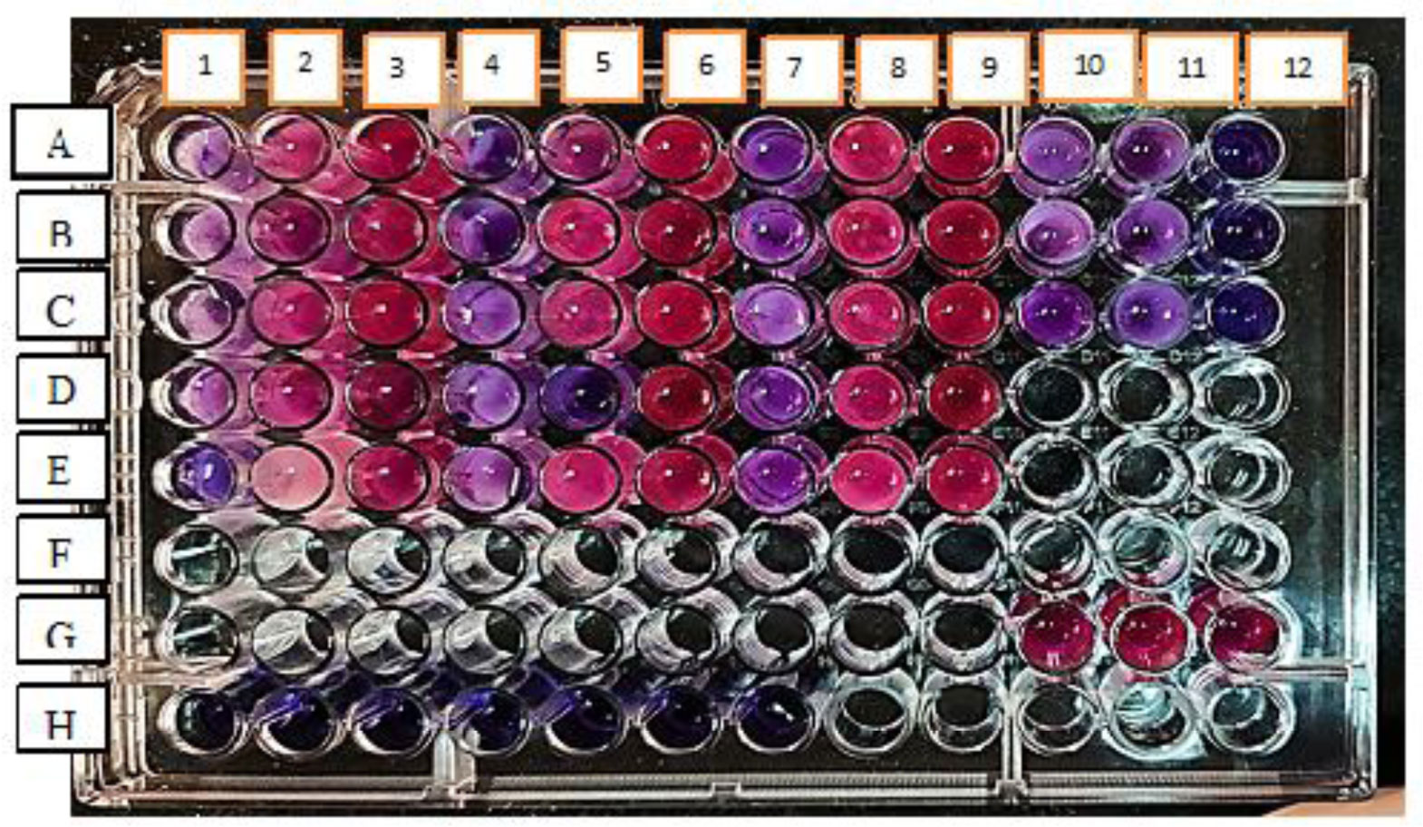
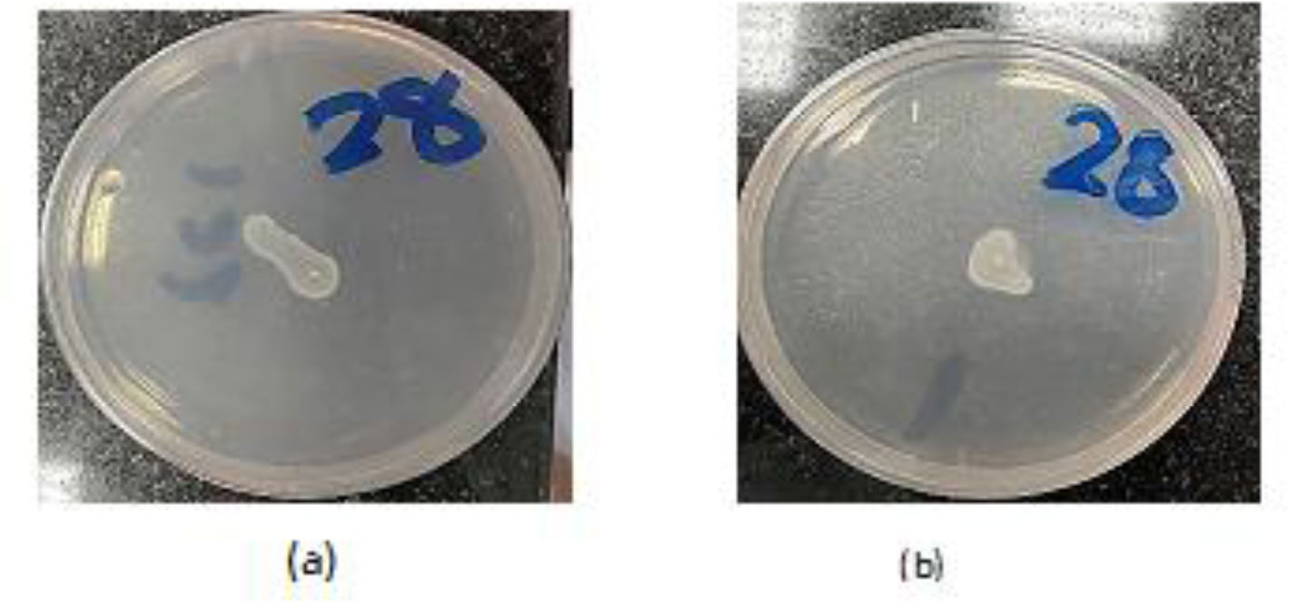
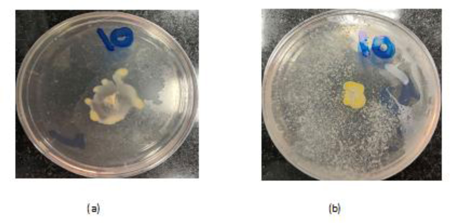
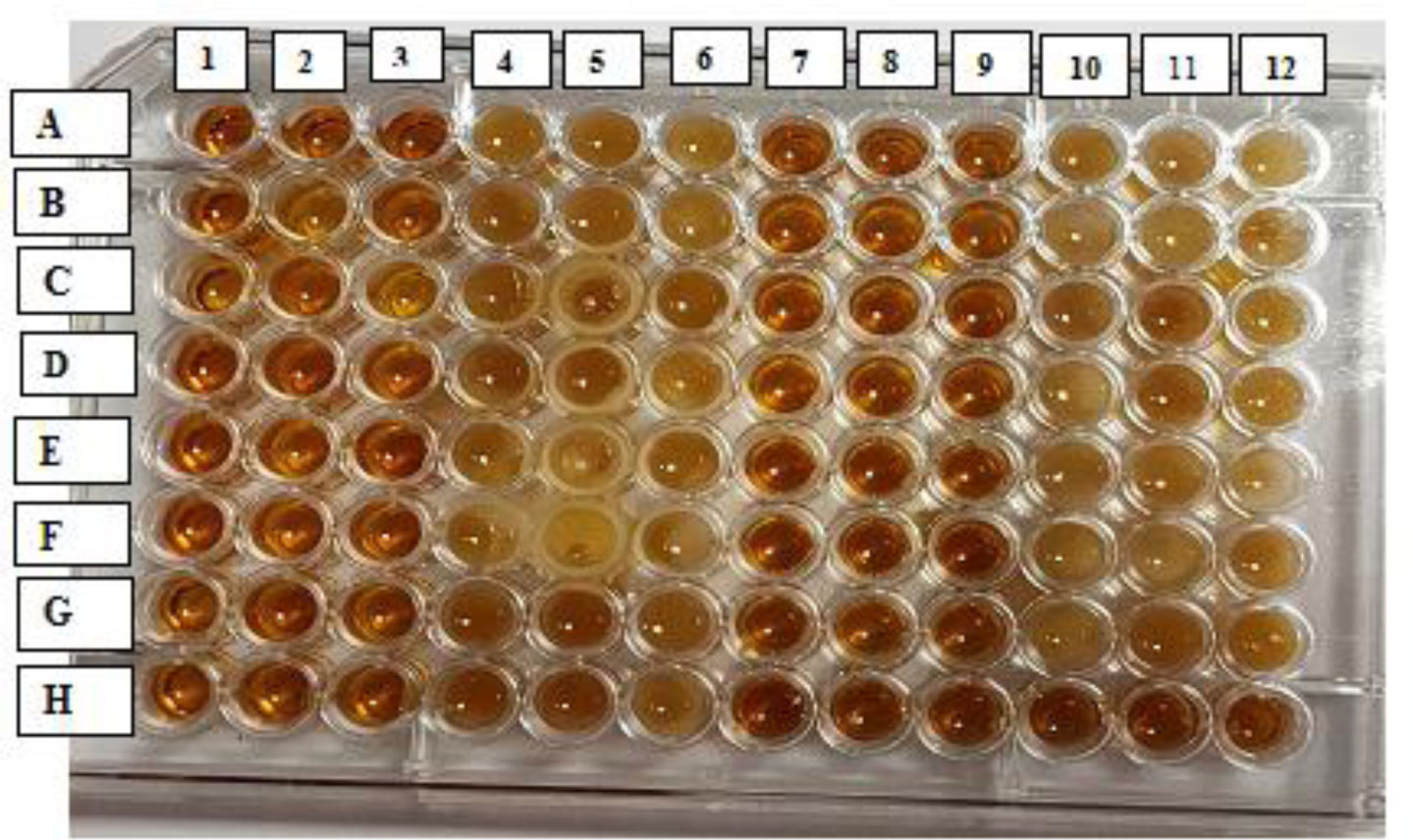
Antibiotic-resistant strains of Pseudomonas aeruginosa (P. aeruginosa) pose a major threat for healthcare-associated and community-acquired infections. P. aeruginosa is recognized as an opportunistic pathogen using quorum sensing (QS) system to regulate the expression of virulence factors and biofilm development. Thus, meddling with the QS system would give alternate methods of controlling the pathogenicity. This study aimed to assess the inhibitory impact of chitosan nanoparticles (CS-NPs) on P. aeruginosa virulence factors regulated by QS (e.g., motility and biofilm formation) and LasI and RhlI gene expression. Minimum inhibitory concentration (MIC) of CS-NPs against 30 isolates of P. aeruginosa was determined. The CS-NPs at sub-MIC were utilized to assess their inhibitory effect on motility, biofilm formation, and the expression levels of LasI and RhlI genes. CS-NPs remarkably inhibited the tested virulence factors as compared to the controls grown without the nanoparticles. The mean (±SD) diameter of swimming motility was decreased from 3.93 (±1.5) to 1.63 (±1.02) cm, and the mean of the swarming motility was reduced from 3.5 (±1.6) to 1.9 (±1.07) cm. All isolates became non-biofilm producers, and the mean percentage rate of biofilm inhibition was 84.95% (±6.18). Quantitative real-time PCR affirmed the opposition of QS activity by lowering the expression levels of LasI and RhlI genes; the expression level was decreased by 90- and 100-folds, respectively. In conclusion, the application of CS-NPs reduces the virulence factors significantly at both genotypic and phenotypic levels. These promising results can breathe hope in the fight against resistant P. aeruginosa by repressing its QS-regulated virulence factors.

| [1] |
Flockton TR, Schnorbus L, Araujo A, et al. (2019) Inhibition of Pseudomonas aeruginosa biofilm formation with surface modified polymeric nanoparticles. Pathogens 8: 55. doi: 10.3390/pathogens8020055

|
| [2] | Cao Q, Wang Y, Chen F, et al. (2014) A novel signal transduction pathway that modulates rhl quorum sensing and bacterial virulence in Pseudomonas aeruginosa. PLoS Pathog 10: 8-10. |
| [3] |
Moradali MF, Ghods S, Rehm BHA (2017) Pseudomonas aeruginosa lifestyle: A paradigm for adaptation, survival, and persistence. Front Cell Infect Microbiol 7. doi: 10.3389/fcimb.2017.00039
|
| [4] |
Kostylev M, Kim DY, Smalley NE, et al. (2019) Evolution of the Pseudomonas aeruginosa quorum-sensing hierarchy. Proc Natl Acad Sci USA 116: 7027-7032. doi: 10.1073/pnas.1819796116
|
| [5] |
Pang Z, Raudonis R, Glick BR, et al. (2019) Antibiotic resistance in Pseudomonas aeruginosa: mechanisms and alternative therapeutic strategies. Biotechnol Adv 37: 177-92. doi: 10.1016/j.biotechadv.2018.11.013
|
| [6] |
Kong M, Chen XG, Xing K, et al. (2010) Antimicrobial properties of chitosan and mode of action: A state of the art review. Int J Food Microbiol 144: 51-63. doi: 10.1016/j.ijfoodmicro.2010.09.012
|
| [7] |
Machul A, Mikołajczyk D, Regiel-Futyra A, et al. (2015) Study on inhibitory activity of chitosan-based materials against biofilm producing Pseudomonas aeruginosa strains. J Biomater Appl 30: 269-278. doi: 10.1177/0885328215578781
|
| [8] |
Ma Z, Garrido-Maestu A, Jeong KC (2017) Application, mode of action, and in vivo activity of chitosan and its micro- and nanoparticles as antimicrobial agents: A review. Carbohydr Polym 176: 257-265. doi: 10.1016/j.carbpol.2017.08.082
|
| [9] |
Vilar Junior JC, Ribeaux DR, Alves Da Silva CA, et al. (2016) Physicochemical and antibacterial properties of chitosan extracted from waste shrimp shells. Int J Microbiol 2016. doi: 10.1155/2016/5127515
|
| [10] |
Chandrasekaran M, Kim KD, Chun SC (2020) Antibacterial activity of chitosan nanoparticles: A review. Processes 8: 1-21. doi: 10.3390/pr8091173
|
| [11] | Tille PM (2017) Traditional cultivation and identification. Bailey and Scott's Diagnostic Microbiology 86-112. |
| [12] | Clinical and Laboratory Standards Institute (2020) CLSI M100 30th Edition. Vol. 30th, Journal of Services Marketing . |
| [13] |
Magiorakos AP, Srinivasan A, Carey RB, et al. (2012) Multidrug-resistant, extensively drug-resistant and pandrug-resistant bacteria: An international expert proposal for interim standard definitions for acquired resistance. Clin Microbiol Infect 18: 268-281. doi: 10.1111/j.1469-0691.2011.03570.x
|
| [14] |
Hasanin MT, Elfeky SA, Mohamed MB, et al. (2018) Production of well-dispersed aqueous cross-linked chitosan-based nanomaterials as alternative antimicrobial approach. J Inorg Organomet Polym Mater 28: 1502-1510. doi: 10.1007/s10904-018-0855-2
|
| [15] |
Elshikh M, Ahmed S, Funston S, et al. (2016) Resazurin-based 96-well plate microdilution method for the determination of minimum inhibitory concentration of biosurfactants. Biotechnol Lett 38: 1015-1019. doi: 10.1007/s10529-016-2079-2
|
| [16] |
Shah S, Gaikwad S, Nagar S, et al. (2019) Biofilm inhibition and anti-quorum sensing activity of phytosynthesized silver nanoparticles against the nosocomial pathogen Pseudomonas aeruginosa. Biofouling 35: 34-49. doi: 10.1080/08927014.2018.1563686
|
| [17] |
Badawy MSEM, Riad OKM, Taher FA, et al. (2020) Chitosan and chitosan-zinc oxide nanocomposite inhibit expression of LasI and RhlI genes and quorum sensing dependent virulence factors of Pseudomonas aeruginosa. Int J Biol Macromol 149: 1109-17. doi: 10.1016/j.ijbiomac.2020.02.019
|
| [18] |
Rehman SA (2018) Comparison of Phenotypic Methods for the Detection of Biofilm Production in Indwelling Medical Devices Used in NICU & PICU in a Tertiary Care Hospital in Hyderabad, India. Int J Curr Microbiol Appl Sci 7: 3265-73. doi: 10.20546/ijcmas.2018.709.405
|
| [19] |
Divya K, Vijayan S, George TK, et al. (2017) Antimicrobial properties of chitosan nanoparticles: Mode of action and factors affecting activity. Fibers Polym 18: 221-230. doi: 10.1007/s12221-017-6690-1
|
| [20] |
Livak KJ, Schmittgen TD (2001) Analysis of relative gene expression data using real-time quantitative PCR and the 2-ΔΔCT method. Methods 25: 402-408. doi: 10.1006/meth.2001.1262
|
| [21] | Hwang W, Yoon SS (2019) Virulence characteristics and an action mode of antibiotic resistance in multidrug-resistant Pseudomonas aeruginosa. Sci Rep 9: 1-15. |
| [22] | Grabski H, Tiratsuyan S (2018) Mechanistic insights of the attenuation of quorum-sensing-dependent virulence factors of Pseudomonas aeruginosa: Molecular modeling of the interaction of taxifolin with transcriptional regulator LasR. bioRxiv 1-31. |
| [23] |
Oliver A, Mulet X, López-Causapé C, et al. (2015) The increasing threat of Pseudomonas aeruginosa high-risk clones. Drug Resist Updat 21–22: 41-59. doi: 10.1016/j.drup.2015.08.002
|
| [24] |
Pérez A, Gato E, Pérez-Llarena J, et al. (2019) High incidence of MDR and XDR Pseudomonas aeruginosa isolates obtained from patients with ventilator-associated pneumonia in Greece, Italy and Spain as part of the MagicBullet clinical trial. J Antimicrob Chemother 74: 1244-52. doi: 10.1093/jac/dkz030
|
| [25] |
Sala A, Ianni F Di, Pelizzone I, et al. (2019) The prevalence of Pseudomonas aeruginosa and multidrug resistant Pseudomonas aeruginosa in healthy captive ophidian. PeerJ 7: 1-13. doi: 10.7717/peerj.6706
|
| [26] | Parmar H, Dholakia A, Vasavada D, et al. (2013) The current status of antibiotic sensitivity of Pseudomonas aeruginosa isolated from various clinical samples. Blood 41: 17.98. |
| [27] |
Pérez-Pérez M, Jorge P, Pérez Rodríguez G, et al. (2017) Quorum sensing inhibition in Pseudomonas aeruginosa biofilms: new insights through network mining. Biofouling 33: 128-42. doi: 10.1080/08927014.2016.1272104
|
| [28] | Zhong L, Ravichandran V, Zhang N, et al. (2020) Attenuation of Pseudomonas aeruginosa quorum sensing by natural products: Virtual screening, evaluation and biomolecular interactions. Int J Mol Sci 21. |
| [29] |
Rozman NAS, Yenn TW, Ring LC, et al. (2019) Potential antimicrobial applications of chitosan nanoparticles (ChNP). J Microbiol Biotechnol 29: 1009-1013. doi: 10.4014/jmb.1904.04065
|
| [30] |
Alqahtani F, Aleanizy F, Tahir E El, et al. (2020) Antibacterial activity of chitosan nanoparticles against pathogenic n. Gonorrhoea. Int J Nanomedicine 15: 7877-7887. doi: 10.2147/IJN.S272736
|
| [31] | Abdeltwab W, Abdelaliem Y, Metry W, et al. (2019) Antimicrobial effect of chitosan and nano-chitosan against some pathogens and spoilage microorganisms. J Adv Lab Res Biol 10: 8-15. |
| [32] | Madhi M, Hasani A, Mojarrad JS, et al. (2020) Impact of chitosan and silver nanoparticles laden with antibiotics on multidrug-resistant Pseudomonas aeruginosa and acinetobacter Baumannii. Arch Clin Infect Dis 15: 1-10. |
| [33] |
Aleanizy FS, Alqahtani FY, Shazly G, et al. (2018) Measurement and evaluation of the effects of pH gradients on the antimicrobial and antivirulence activities of chitosan nanoparticles in Pseudomonas aeruginosa. Saudi Pharm J 26: 79-83. doi: 10.1016/j.jsps.2017.10.009
|
| [34] | Limoli DH, Warren EA, Yarrington KD, et al. (2019) Interspecies interactions induce exploratory motility in Pseudomonas aeruginosa. eLifeMicrobiology Infect Dis 8: 1-24. |
| [35] | Leighton TL, Harvey H, Howell PL, et al. (2017) Cyclic AMP-independent control of twitching motility in Pseudomonas aeruginosa. J Bacteriol 199: 1-14. |
| [36] |
Heydorn A, Ersbøll B, Kato J, et al. (2002) Statistical analysis of Pseudomonas aeruginosa biofilm development: Impact of mutations in genes involved in twitching motility, cell-to-cell signaling, and stationary-phase sigma factor expression. Appl Environ Microbiol 68: 2008-2017. doi: 10.1128/AEM.68.4.2008-2017.2002
|
| [37] |
Khan F, Manivasagan P, Thuy D, et al. (2019) Microbial pathogenesis antibiofilm and antivirulence properties of chitosan-polypyrrole nanocomposites to Pseudomonas aeruginosa. Microb Pthogenes 128: m363-73. doi: 10.1016/j.micpath.2019.01.033
|
| [38] |
Rubini D, Farisa S, Subramani P (2019) Extracted chitosan disrupts quorum sensing mediated virulence factors in Urinary tract infection causing pathogens. Pathog Dis 77. doi: 10.1093/femspd/ftz009
|
| [39] | Davies DG, Parsek MR, Pearson JP, et al. (1998) The involvement of cell-to-cell signals in the development of a bacterial biofilm. AAAS 280: 295-299. |
| [40] |
Colvin KM, Irie Y, Tart CS, et al. (2012) The Pel and Psl polysaccharides provide Pseudomonas aeruginosa structural redundancy within the biofilm matrix. Environ Microbiol 14: 1913-1928. doi: 10.1111/j.1462-2920.2011.02657.x
|
| [41] |
Muslim SN, Kadmy IMSA, Ali ANM, et al. (2018) Chitosan extracted from Aspergillus flavus shows synergistic effect, eases quorum sensing mediated virulence factors and biofilm against nosocomial pathogen Pseudomonas aeruginosa. Int J Biol Macromol 107: 52-58. doi: 10.1016/j.ijbiomac.2017.08.146
|
| [42] |
Vaidyanathan R, Gopalram S, Kalishwaralal K, et al. (2010) Enhanced silver nanoparticle synthesis by optimization of nitrate reductase activity. Colloids Surfaces B Biointerfaces 75: 335-41. doi: 10.1016/j.colsurfb.2009.09.006
|
| [43] |
Mukherjee S, Moustafa D, Smith CD, et al. (2017) The RhlR quorum-sensing receptor controls Pseudomonas aeruginosa pathogenesis and biofilm development independently of its canonical homoserine lactone autoinducer. PLOS Pathog 13: 1-25. doi: 10.1371/journal.ppat.1006504
|
| [44] |
Landriscina A, Rosen J, Friedman AJ (2015) Biodegradable chitosan nanoparticles in drug delivery for infectious disease. Nanomedicine 10: 1609-1619. doi: 10.2217/nnm.15.7
|
| [45] |
Qi L, Xu Z, Jiang X, et al. (2004) Preparation and antibacterial activity of chitosan nanoparticles. Carbohydr Res 339: 2693-2700. doi: 10.1016/j.carres.2004.09.007
|
Figures(7) / Tables(2)

Rana Abdel Fattah Abdel Fattah, Fatma El zaharaa Youssef Fathy, Tahany Abdel Hamed Mohamed, Marwa Shabban Elsayed. Effect of chitosan nanoparticles on quorum sensing-controlled virulence factors and expression of LasI and RhlI genes among Pseudomonas aeruginosa clinical isolates[J]. AIMS Microbiology, 2021, 7(4): 415-430. doi: 10.3934/microbiol.2021025


 DownLoad: