This study compared the dose enhancement predicted in kilovoltage gold nanoparticle-enhanced radiotherapy using the newly developed EGS lattice and the typical gold-water mixture method in Monte Carlo simulation. This new method considered the gold nanoparticle-added volume consisting of solid nanoparticles instead of a gold-water mixture. In addition, this particle method is more realistic in simulation.
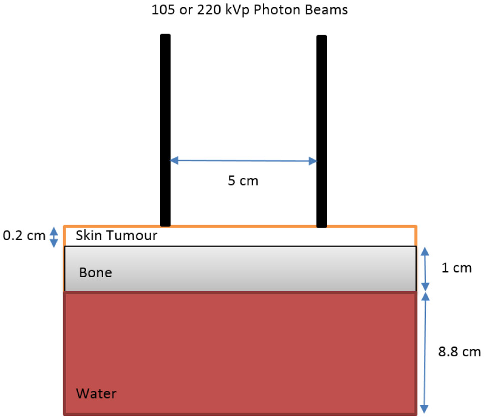
A heterogeneous phantom containing bone and water was irradiated by the 105 and 220 kVp x-ray beams. Gold nanoparticles were added to the tumour volume with concentration varying from 3–40 mg/mL in the phantom. The dose enhancement ratio (DER), defined as the ratio of dose at the tumour with and without adding gold nanoparticles, was calculated by the gold-water mixture and particle method using Monte Carlo simulation for comparison.
It is found that the DER was 1.44–4.71 (105 kVp) and 1.27–2.43 (220 kVp) for the gold nanoparticle concentration range of 3–40 mg/mL, when they were calculated by the gold-water mixture method. The DER was slightly larger and equal to 1.47–4.84 (105 kVp) and 1.29–2.5 (220 kVp) for the same concentration range, when the particle method was used. Moreover, the DER predicted by both methods increased with an increase of nanoparticle concentration, and a decrease of x-ray beam energy.
The deviation of DER determined by the particle and gold-water mixture method was insignificant when considering the uncertainty in the calculation of DER (2%) in the nanoparticle concentration range of 3–40 mg/mL. It is therefore concluded that the gold-water mixture method could predict the dose enhancement as accurate as the newly developed particle method.
Citation: Zaynah Sheeraz, James C.L. Chow. Evaluation of dose enhancement with gold nanoparticles in kilovoltage radiotherapy using the new EGS geometry library in Monte Carlo simulation[J]. AIMS Biophysics, 2021, 8(4): 337-345. doi: 10.3934/biophy.2021027
This study compared the dose enhancement predicted in kilovoltage gold nanoparticle-enhanced radiotherapy using the newly developed EGS lattice and the typical gold-water mixture method in Monte Carlo simulation. This new method considered the gold nanoparticle-added volume consisting of solid nanoparticles instead of a gold-water mixture. In addition, this particle method is more realistic in simulation.
A heterogeneous phantom containing bone and water was irradiated by the 105 and 220 kVp x-ray beams. Gold nanoparticles were added to the tumour volume with concentration varying from 3–40 mg/mL in the phantom. The dose enhancement ratio (DER), defined as the ratio of dose at the tumour with and without adding gold nanoparticles, was calculated by the gold-water mixture and particle method using Monte Carlo simulation for comparison.
It is found that the DER was 1.44–4.71 (105 kVp) and 1.27–2.43 (220 kVp) for the gold nanoparticle concentration range of 3–40 mg/mL, when they were calculated by the gold-water mixture method. The DER was slightly larger and equal to 1.47–4.84 (105 kVp) and 1.29–2.5 (220 kVp) for the same concentration range, when the particle method was used. Moreover, the DER predicted by both methods increased with an increase of nanoparticle concentration, and a decrease of x-ray beam energy.
The deviation of DER determined by the particle and gold-water mixture method was insignificant when considering the uncertainty in the calculation of DER (2%) in the nanoparticle concentration range of 3–40 mg/mL. It is therefore concluded that the gold-water mixture method could predict the dose enhancement as accurate as the newly developed particle method.

| [1] | Khan FM, Gibbons JP, Sperduto PW (2016) Khan's Treatment Planning in Radiation Oncology Wolters Kluwer. |
| [2] |
Antoine M, Ralite F, Soustiel C, et al. (2019) Use of metrics to quantify IMRT and VMAT treatment plan complexity: A systematic review and perspectives. Phys Med 64: 98-108. doi: 10.1016/j.ejmp.2019.05.024

|
| [3] |
Bortfeld T (2006) IMRT: a review and preview. Phys Med Biol 51: R363-379. doi: 10.1088/0031-9155/51/13/R21
|
| [4] |
Staffurth J (2010) A review of the clinical evidence for intensity-modulated radiotherapy. Clin Oncol 22: 643-657. doi: 10.1016/j.clon.2010.06.013
|
| [5] |
Penninckx S, Heuskin AC, Michiels C, et al. (2020) Gold nanoparticles as a potent radiosensitizer: A transdisciplinary approach from physics to patient. Cancers 12: 2021. doi: 10.3390/cancers12082021
|
| [6] |
Siddique S, Chow JCL (2020) Gold nanoparticles for drug delivery and cancer therapy. App Sci 10: 3824. doi: 10.3390/app10113824
|
| [7] |
Moore JA, Chow JCL (2021) Recent progress and applications of gold nanotechnology in medical biophysics using artificial intelligence and mathematical modeling. Nano Ex 2: 022001. doi: 10.1088/2632-959X/abddd3
|
| [8] | Abolfazli MK, Mahdavi SR, Ataei G (2015) Studying effects of gold nanoparticle on dose enhancement in megavoltage radiation. J Biomed Phys Eng 5: 185-190. |
| [9] |
Kuncic Z, Lacombe S (2018) Nanoparticle radio-enhancement: principles, progress and application to cancer treatment. Phys Med Biol 63: 02TR01. doi: 10.1088/1361-6560/aa99ce
|
| [10] |
Li W, Zhao X, Du B, et al. (2016) Gold nanoparticle–mediated targeted delivery of recombinant human endostatin normalizes tumour vasculature and improves cancer therapy. Sci Rep 6: 1-11. doi: 10.1038/s41598-016-0001-8
|
| [11] |
Grzelczak M, Pérez-Juste J, Mulvaney P, et al. (2008) Shape control in gold nanoparticle synthesis. Chem Soc Rev 37: 1783-1791. doi: 10.1039/b711490g
|
| [12] |
Liu XY, Wang JQ, Ashby CR, et al. (2021) Gold nanoparticles: synthesis, physiochemical properties and therapeutic applications in cancer. Drug Discov Today 26: 1284-1292. doi: 10.1016/j.drudis.2021.01.030
|
| [13] |
Engels E, Bakr S, Bolst D, et al. (2020) Advances in modelling gold nanoparticle radiosensitization using new Geant4-DNA physics models. Phys Med Biol 65: 225017. doi: 10.1088/1361-6560/abb7c2
|
| [14] |
Torrisi L (2021) Physical aspects of gold nanoparticles as cancer killer therapy. Ind J Phys 95: 225-234. doi: 10.1007/s12648-019-01679-1
|
| [15] |
Ahn S, Jung SY, Lee SJ (2013) Gold nanoparticle contrast agents in advanced X-ray imaging technologies. Molecules 18: 5858-5890. doi: 10.3390/molecules18055858
|
| [16] |
Dong YC, Hajfathalian M, Maidment PSN, et al. (2019) Effect of gold nanoparticle size on their properties as contrast agents for computed tomography. Sci Rep 9: 14912. doi: 10.1038/s41598-019-50332-8
|
| [17] |
Jain S, Hirst DG, O'sullivan JM (2012) Gold nanoparticles as novel agents for cancer therapy. Brit J Radiol 85: 101-113. doi: 10.1259/bjr/59448833
|
| [18] |
Bobo D, Robinson KJ, Islam J, et al. (2016) Nanoparticle-based medicines: a review of FDA-approved materials and clinical trials to date. Pharm Res 33: 2373-2387. doi: 10.1007/s11095-016-1958-5
|
| [19] |
Siddique S, Chow JCL (2020) Application of nanomaterials in biomedical imaging and cancer therapy. Nanomaterials 10: 1700. doi: 10.3390/nano10091700
|
| [20] |
Butterworth KT, Nicol JR, Ghita M, et al. (2016) Preclinical evaluation of gold-DTDTPA nanoparticles as theranostic agents in prostate cancer radiotherapy. Nanomedicine 11: 2035-2047. doi: 10.2217/nnm-2016-0062
|
| [21] |
Chow JCL (2020) Depth dose enhancement on flattening-filter-free X-ray beam: A Monte Carlo study in nanoparticle-enhanced radiotherapy. App Sci 10: 7052. doi: 10.3390/app10207052
|
| [22] |
Kakade NR, Sharma SD (2015) Dose enhancement in gold nanoparticle-aided radiotherapy for the therapeutic X-ray beams using Monte Carlo technique. J Cancer Res Ther 11: 94. doi: 10.4103/0973-1482.147691
|
| [23] |
Jones BL, Krishnan S, Cho SH (2010) Estimation of microscopic dose enhancement factor around gold nanoparticles by Monte Carlo calculations. Med Phys 37: 3809-3816. doi: 10.1118/1.3455703
|
| [24] |
Cho SH (2005) Estimation of tumour dose enhancement due to gold nanoparticles during typical radiation treatments: a preliminary Monte Carlo study. Phys Med Biol 50: N163. doi: 10.1088/0031-9155/50/15/N01
|
| [25] |
Rogers DWO (2006) Fifty years of Monte Carlo simulations for medical physics. Phys Med Biol 51: R287. doi: 10.1088/0031-9155/51/13/R17
|
| [26] |
Miras H, Jiménez R, Miras C, et al. (2013) CloudMC: a cloud computing application for Monte Carlo simulation. Phys Med Biol 58: N125-N133. doi: 10.1088/0031-9155/58/8/N125
|
| [27] |
Chun H, Chow JCL (2016) Gold nanoparticle DNA damage in radiotherapy: A Monte Carlo study. AIMS Bioeng 3: 352-361. doi: 10.3934/bioeng.2016.3.352
|
| [28] |
Poignant F, Monini C, Testa É, et al. (2021) Influence of gold nanoparticles embedded in water on nanodosimetry for keV photon irradiation. Med Phys 48: 1874-1883. doi: 10.1002/mp.14576
|
| [29] |
Chow JCL (2018) Recent progress in Monte Carlo simulation on gold nanoparticle radiosensitization. AIMS Biophys 5: 231-244. doi: 10.3934/biophy.2018.4.231
|
| [30] |
Incerti S, Baldacchino G, Bernal M, et al. (2010) The geant4-dna project. Int J Model Simul Sci Comp 1: 157-178. doi: 10.1142/S1793962310000122
|
| [31] |
Martelli S, Chow JCL (2020) Dose enhancement for the flattening-filter-free and flattening-filter X-ray beams in nanoparticle-enhanced radiotherapy: A Monte Carlo phantom study. Nanomaterials 10: 637. doi: 10.3390/nano10040637
|
| [32] |
Zheng XJ, Chow JCL (2017) Radiation dose enhancement in skin therapy with nanoparticle addition: A Monte Carlo study on kilovoltage photon and megavoltage electron beams. World J Radiol 9: 63-71. doi: 10.4329/wjr.v9.i2.63
|
| [33] |
Koger B, Kirkby C (2016) A method for converting dose-to-medium to dose-to-tissue in Monte Carlo studies of gold nanoparticle-enhanced radiotherapy. Phys Med Biol 61: 2014. doi: 10.1088/0031-9155/61/5/2014
|
| [34] |
Kawrakow I (2000) Accurate condensed history Monte Carlo simulation of electron transport. I. EGSnrc, the new EGS4 version. Med Phys 27: 485-498. doi: 10.1118/1.598917
|
| [35] |
Martinov MP, Thomson RM (2020) Taking EGSnrc to new lows: Development of egs++ lattice geometry and testing with microscopic geometries. Med Phys 47: 3225-3232. doi: 10.1002/mp.14172
|
| [36] | International ommission on Radiation Units and Measurements Tissue substitutes in radiation dosimetry and measurements, United States (1989) . |
| [37] | Kawrakow I (2005) egspp: the EGSnrc C++ class library. Technical Report, PIRS-899 National Research Council Canada: Ottawa, Canada. |
| [38] | Rogers DWO, Walters B, Kawrakow I (2009) BEAMnrc users manual. NRC Report PIRS 509: 12. |
| [39] |
Hainfeld JF, Slatkin DN, Smilowitz HM (2004) The use of gold nanoparticles to enhance radiotherapy in mice. Phys Med Biol 49: N309. doi: 10.1088/0031-9155/49/18/N03
|
| [40] | Rogers DWO, Kawrakow I, Seuntjens JP, et al. (2003) NRC user codes for EGSnrc: NRC Technical Report PIRS 702 (rev C) National Research Council Canada: Ottawa, Canada. |
| [41] | Walters BR, Kawrakow I, Rogers DWO (2005) DOSXYZnrc users manual. NRC Report PIRS 794: 57-58. |

Figures(2)

Zaynah Sheeraz, James C.L. Chow. Evaluation of dose enhancement with gold nanoparticles in kilovoltage radiotherapy using the new EGS geometry library in Monte Carlo simulation[J]. AIMS Biophysics, 2021, 8(4): 337-345. doi: 10.3934/biophy.2021027


 DownLoad: