


Figure 1.
Function h in definition (5.1).
Given two digital images (Xi,ki),i∈{1,2}, first of all we establish a new PNk-adjacency relation in a digital product X1×X2 to obtain a relation set (X1×X2,PNk), where the term ″PN" means ″pseudo-normal". Indeed, a PN-k-adjacency is softer or broader than a normal k-adjacency. Next, the present paper initially develops both PN-k-continuity and PN-k-isomorphism. Furthermore, it proves that these new concepts, the PN-k-continuity and PN-k-isomorphism, need not be equal to the typical k-continuity and a k-isomorphism, respectively. Precisely, we prove that none of the typical k-continuity (resp. typical k-isomorphism) and the PN-k-continuity (resp. PN-k-isomorphism) implies the other. Then we prove that for each i∈{1,2}, the typical projection map Pi:X1×X2→Xi preserves a PNk-adjacency relation in X1×X2 to the ki-adjacency relation in (Xi,ki). In particular, using a PN-k-isomorphism, we can classify digital products with PNk-adjacencies. Furthermore, in the category of digital products with PNk-adjacencies and PN-k-continuous maps between two digital products with PNk-adjacencies, denoted by DTC▴k, we finally study the (almost) fixed point property of (X1×X2,PNk).
Citation: Jeong Min Kang, Sang-Eon Han, Sik Lee. Digital products with PNk-adjacencies and the almost fixed point property in DTC▴k[J]. AIMS Mathematics, 2021, 6(10): 11550-11567. doi: 10.3934/math.2021670
| [1] | A. Vinodkumar, T. Senthilkumar, S. Hariharan, J. Alzabut . Exponential stabilization of fixed and random time impulsive delay differential system with applications. Mathematical Biosciences and Engineering, 2021, 18(3): 2384-2400. doi: 10.3934/mbe.2021121 |
| [2] | Eduardo Liz, Alfonso Ruiz-Herrera . Delayed population models with Allee effects and exploitation. Mathematical Biosciences and Engineering, 2015, 12(1): 83-97. doi: 10.3934/mbe.2015.12.83 |
| [3] | Paolo Fergola, Marianna Cerasuolo, Edoardo Beretta . An allelopathic competition model with quorum sensing and delayed toxicant production. Mathematical Biosciences and Engineering, 2006, 3(1): 37-50. doi: 10.3934/mbe.2006.3.37 |
| [4] | Yoichi Enatsu, Yukihiko Nakata, Yoshiaki Muroya . Global stability for a class of discrete SIR epidemic models. Mathematical Biosciences and Engineering, 2010, 7(2): 347-361. doi: 10.3934/mbe.2010.7.347 |
| [5] | Xinran Zhou, Long Zhang, Tao Zheng, Hong-li Li, Zhidong Teng . Global stability for a class of HIV virus-to-cell dynamical model with Beddington-DeAngelis functional response and distributed time delay. Mathematical Biosciences and Engineering, 2020, 17(5): 4527-4543. doi: 10.3934/mbe.2020250 |
| [6] | Hongjing Shi, Wanbiao Ma . An improved model of t cell development in the thymus and its stability analysis. Mathematical Biosciences and Engineering, 2006, 3(1): 237-248. doi: 10.3934/mbe.2006.3.237 |
| [7] | Marion Weedermann . Analysis of a model for the effects of an external toxin on anaerobic digestion. Mathematical Biosciences and Engineering, 2012, 9(2): 445-459. doi: 10.3934/mbe.2012.9.445 |
| [8] | Kalyan Manna, Malay Banerjee . Stability of Hopf-bifurcating limit cycles in a diffusion-driven prey-predator system with Allee effect and time delay. Mathematical Biosciences and Engineering, 2019, 16(4): 2411-2446. doi: 10.3934/mbe.2019121 |
| [9] | C. Connell McCluskey . Global stability of an SIR epidemic model with delay and general nonlinear incidence. Mathematical Biosciences and Engineering, 2010, 7(4): 837-850. doi: 10.3934/mbe.2010.7.837 |
| [10] | Jinliang Wang, Hongying Shu . Global analysis on a class of multi-group SEIR model with latency and relapse. Mathematical Biosciences and Engineering, 2016, 13(1): 209-225. doi: 10.3934/mbe.2016.13.209 |
Given two digital images (Xi,ki),i∈{1,2}, first of all we establish a new PNk-adjacency relation in a digital product X1×X2 to obtain a relation set (X1×X2,PNk), where the term ″PN" means ″pseudo-normal". Indeed, a PN-k-adjacency is softer or broader than a normal k-adjacency. Next, the present paper initially develops both PN-k-continuity and PN-k-isomorphism. Furthermore, it proves that these new concepts, the PN-k-continuity and PN-k-isomorphism, need not be equal to the typical k-continuity and a k-isomorphism, respectively. Precisely, we prove that none of the typical k-continuity (resp. typical k-isomorphism) and the PN-k-continuity (resp. PN-k-isomorphism) implies the other. Then we prove that for each i∈{1,2}, the typical projection map Pi:X1×X2→Xi preserves a PNk-adjacency relation in X1×X2 to the ki-adjacency relation in (Xi,ki). In particular, using a PN-k-isomorphism, we can classify digital products with PNk-adjacencies. Furthermore, in the category of digital products with PNk-adjacencies and PN-k-continuous maps between two digital products with PNk-adjacencies, denoted by DTC▴k, we finally study the (almost) fixed point property of (X1×X2,PNk).
In this paper, we study the following general class of functional differential equations with distributed delay and bistable nonlinearity,
| {x′(t)=−f(x(t))+∫τ0h(a)g(x(t−a))da,t>0,x(t)=ϕ(t),−τ≤t≤0. | (1.1) |
Many mathematical models issued from ecology, population dynamics and other scientific fields take the form of Eq (1.1) (see, e.g., [1,2,3,4,5,6,7,8,9,10,11,12,13,14,15] and references therein). When a spatial diffusion is considered, many models are studied in the literature (see, e.g., [16,17,18,19,20,21,22]).
For the case where g(x)=f(x) has not only the trivial equilibrium but also a unique positive equilibrium, Eq (1.1) is said to be a problem with monostable nonlinearity. In this framework, many authors studied problem (1.1) with various monostable nonlinearities such as Blowflies equations, where f(x)=μx and g(x)=βxe−αx, and Mackey-Glass equations, where f(x)=μx and g(x)=βx/(α+xn) (see, e.g., [1,3,6,7,9,10,11,12,13,21,23,24,25,26,27]).
When g(x) allows Eq (1.1) to have two positive equilibria x∗1 and x∗2 in addition to the trivial equilibrium, Eq (1.1) is said to be a problem with bistable nonlinearity. In this case, Huang et al. [5] investigated the following general equation:
| x′(t)=−f(x(t))+g(x(t−τ)). |
The authors described the basins of attraction of equilibria and obtained a series of invariant intervals using the decomposition domain. Their results were applied to models with Allee effect, that is, f(x)=μx and g(x)=βx2e−αx. We point out that the authors in [5] only proved the global stability for x∗2≤M, where g(M)=maxs∈R+g(s). In this paper, we are interested in the dynamics of the bistable nonlinearity problem (1.1). More precisely, we will present some attracting intervals which will enable us to give general conditions on f and g that ensure global asymptotic stability of equilibria x∗1 and x∗2 in the both cases x∗2<M and x∗2≥M.
The paper is organized as follows: in Section 2, we give some preliminary results including existence, uniqueness and boundedness of the solution as well as a comparison result. We finish this section by proving the global asymptotic stability of the trivial equilibrium. Section 3 is devoted to establish the attractive intervals of solutions and to prove the global asymptotic stability of the positive equilibrium x∗2. In Section 4, we investigate an application of our results to a model with Allee effect. In Section 5, we perform numerical simulation that supports our theoretical results. Finally, Section 6 is devoted to the conclusion.
In the whole paper, we suppose that the function h is positive and
| ∫τ0h(a)da=1. |
We give now some standard assumptions.
(T1) f and g are Lipschitz continuous with f(0)=g(0)=0 and there exists a number B>0 such that maxv∈[0,s]g(v)<f(s) for all s>B.
(T2) f′(s)>0 for all s≥0.
(T3) g(s)>0 for all s>0 and there exists a unique M>0 such that g′(s)>0 for 0<s<M, g′(M)=0 and g′(s)<0 for s>M.
(T4) There exist two positive constants x∗1 and x∗2 such that g(x)<f(x) if x∈(0,x∗1)∪(x∗2,∞) and g(x)>f(x) if x∈(x∗1,x∗2) and g′(x∗1)>f′(x∗1).
Let C:=C([−τ,0],R) be the Banach space of continuous functions defined in [−τ,0] with ||ϕ||=supθ∈[−τ,0]|ϕ(θ)| and C+={ϕ∈C;ϕ(θ)≥0,−τ≤θ≤0} is the positive cone of C. Then, (C,C+) is a strongly ordered Banach space. That is, for all ϕ,ψ∈C, we write ϕ≥ψ if ϕ−ψ∈C+, ϕ>ψ if ϕ−ψ∈C+∖{0} and ϕ>>ψ if ϕ−ψ∈Int(C+). We define the following ordered interval:
| C[ϕ,ψ]:={ξ∈C;ϕ≤ξ≤ψ}. |
For any χ∈R, we write χ∗ for the element of C satisfying χ∗(θ)=χ for all θ∈[−τ,0]. The segment xt∈C of a solution is defined by the relation xt(θ)=x(t+θ), where θ∈[−τ,0] and t≥0. In particular, x0=ϕ. The family of maps
| Φ:[0,∞)×C+→C+, |
such that
| (t,ϕ)→xt(ϕ) |
defines a continuous semiflow on C+ [28]. For each t≥0, the map Φ(t,.) is defined from C+ to C+ which is denoted by Φt:
| Φt(ϕ)=Φ(t,ϕ). |
The set of equilibria of the semiflow, which is generated by (1.1), is given by
| E={χ∗∈C+;χ∈Randg(χ)=f(χ)}. |
In this section, we first provide existence, uniqueness and boundedness of solution to problem (1.1). We then present a Lyapunov functional and show the global asymptotic stability of the trivial equilibrium. We begin by recalling a useful theorem related to a comparison principle (see Theorem 1.1 in page 78 in [29]).
We consider the following problem:
| {x′(t)=F(xt),t>0,x(t)=ϕ(t),−τ≤t≤0, | (2.1) |
where F:Ω→R is continuous on Ω, which is an open subset of C. We write x(t,ϕ,F) for the maximal defined solution of problem (2.1). When we need to emphasize the dependence of a solution on initial data, we write x(t,ϕ) or x(ϕ).
Theorem 2.1. Let f1, f2 :Ω→R be continuous, Lipschitz on each compact subset of Ω, and assume that either f1 or f2 is a nondecreasing function, with f1(ϕ)≤f2(ϕ) for all ϕ∈Ω. Then
| x(t,ϕ,f1)≤x(t,ϕ,f2), |
holds for all t≥0, for which both are defined.
The following lemma states existence, uniqueness and boundedness of the positive solution to problem (1.1). For the proof, see [15,30,31].
Lemma 2.2. Suppose that (T1) holds. For any ϕ∈C+, the problem (1.1) has a unique positive solution x(t):=x(t,ϕ) on [0,∞) satisfying x0=ϕ, provided ϕ(0)>0. In addition, we have the following estimate:
| 0≤lim supt→∞x(t)≤B. |
Moreover, the semiflow Φt admits a compact global attractor, which attracts every bounded set in C+.
The following lemma can be easily proved (see also the proof of Theorem 1.1 in [29]).
Lemma 2.3. Let ϕ∈C be a given initial condition, x(ϕ) be the solution of problem (1.1) and xϵ(ϕ), ϵ>0 be the solution of problem (1.1) when replacing f by f±ϵ. Then
| xϵ(t,ϕ)→x(t,ϕ) as ϵ→0, for all t∈[0,∞). |
We focus now on the global stability of the trivial equilibrium. For this purpose, we suppose that
| f(s)>g(s) for all s∈(0,x∗1) and f(x∗1)=g(x∗1). | (2.2) |
Lemma 2.4. Assume that (T1) and condition (2.2) hold. For a given ϕ∈C[0,x∗1]∖{x∗1}, the solution x(ϕ) of problem (1.1) satisfies
| lim supt→∞x(t)<x∗1, | (2.3) |
provided that one of the following hypotheses holds:
(i) g is a nondecreasing function over (0,x∗1).
(ii) f is a nondecreasing function over (0,x∗1).
Proof. Without loss of generality, we assume that ϕ(0)<x∗1. Suppose that (ⅰ) holds. We first claim that x(t)<x∗1 for all t≥0. Let xϵ(ϕ) be the solution of problem (1.1) by replacing f by f+ϵ. We prove that xϵ(t):=xϵ(t,ϕ)≤x∗1 for all t>0. Suppose, on the contrary, that there exists t1>0 such that xϵ(t1)=x∗1, xϵ(t)≤x∗1 for all t≤t1 and x′ϵ(t1)≥0. Then, using the equation of xϵ(t1), we have
| 0≤x′ϵ(t1)=−f(xϵ(t1))−ϵ+∫τ0h(a)g(xϵ(t1−a))da,<−f(x∗1)+g(x∗1)=0, |
which leads to a contradiction. Now, applying Lemma 2.3, we obtain x(t)≤x∗1 for all t≥0. Next, set X(t)=x∗1−x(t). We then have
| X′(t)=f(x(t))−f(x∗1)+∫τ0h(a)(g(x∗1)−g(x(t−a)))da. |
Since x(t)≤x∗1 for all t≥0 and g is a nondecreasing function, we have, for t≥τ,
| X′(t)≥−LX(t), |
where L is the Lipschitz constant of f. Consequently, X(t)≥X(0)e−Lt and the claim is proved. Finally, to prove inequality (2.3), we suppose, on the contrary, that there exist an increasing sequence (tn)n, tn→∞, t0≥τ and a nondecreasing sequence (x(tn))n, such that x(tn)→x∗1 as tn→∞, x(tn)<x∗1 for some n and x(tn)=maxt∈[0,tn]x(t). Then, in view of condition (2.2), the equation of x(tn) satisfies
| 0≤x′(tn)=−f(x(tn))+∫τ0h(a)g(x(tn−a))da,≤−f(x(tn))+g(x(tn))<0, |
which is a contradiction.
Suppose now that (ⅱ) holds. Let xϵ(t) be the solution of problem (1.1) by replacing f(s) by f(s)+ϵ and g(s) by g+(s)=maxσ∈[0,s]g(σ).
Then, again by contradiction, suppose that there exists t1>0 such that xϵ(t1)=x∗1, xϵ(t)≤x∗1 for all t≤t1 and x′ϵ(t1)≥0. Then, arguing as above, we obtain
| 0≤x′ϵ(t1)=−f(xϵ(t1))−ϵ+∫τ0h(a)g+(xϵ(t−a))da,<−f(x∗1)+g+(x∗1). | (2.4) |
Since f is a nondecreasing function and g+ is the smallest nondecreasing function that is greater than g, we obtain f(s)>g+(s) for all s∈(0,x∗1). This contradicts with inequality (2.4). Further, by combining Theorem 2.1 and Lemma 2.3, we get x(t)≤x∗1 for all t≥0. Finally, following the same arguments as in the first part of this proof, the lemma is proved.
We now prove the global asymptotic stability of the trivial equilibrium.
Theorem 2.5. Assume that (T1) and condition (2.2) hold. Suppose also that ϕ∈C[0,x∗1]∖{x∗1}. The trivial equilibrium is globally asymptotically stable if one of the following hypotheses holds:
(i) g is a nondecreasing function over (0,x∗1).
(ii) f is a nondecreasing function over (0,x∗1).
Proof. Suppose that (ⅰ) holds. Let V be the Lyapunov functional defined by
| V(s)=s+∫τ0ψ(a)g(ϕ(−a))da, | (2.5) |
where ψ(a)=∫τah(σ)dσ. The derivative of V along the solution of problem (1.1) gives
| dV(xt)dt=g(x(t))−f(x(t))∀t>0. |
From condition (2.2) and Lemma 2.4, we have dV(xt)/dt<0 and thus, the result is reached by classical Lyapunov theorem (see [6]). Next, suppose that (ⅱ) holds. Let the function V be defined in (2.5) by replacing g(s) by g+(s):=maxσ∈[0,s]g(σ). Since g+(s)<f(s) for all s∈(0,x∗1), we can employ the same argument as above to get dV(xt)/dt<0. Finally the result is obtained by applying Theorem 2.1 and Lemma 2.4. This completes the proof.
Now, suppose that
| f(s)>g(s) for all s>0. | (2.6) |
Using the same proof as in Theorem 2.5, we immediately obtain the following theorem.
Theorem 2.6. Assume that (T1) and condition (2.6) hold. The trivial equilibrium is globally asymptotically stable for all ϕ∈C+.
The following theorem concerns the global stability of x∗2 in the case where g is a nondecreasing function.
Theorem 3.1. Suppose that ϕ∈C[x∗1,sups∈[−τ,0]ϕ]∖{x∗1} and g is a nondecreasing function. Assume also that (T1) and (T4) hold. Then, the positive equilibrium x∗2 is globally asymptotically stable.
Proof. Without loss of generality, suppose that ϕ(0)>x∗1. We first claim that lim inft→∞x(t)>x∗1. For this, let xϵ(t):=xϵ(t;ϕ) be the solution of problem (1.1) when replacing f by f−ϵ. To reach the claim, we begin by proving that xϵ(t)>x∗1 for all t≥0. Otherwise, there exists t1>0 such that xϵ(t1)=x∗1, xϵ(t)≥x∗1 for all t≤t1 and x′ϵ(t1)≤0. Then, the equation of xϵ(t1) satisfies
| 0≥x′ϵ(t1)=−f(xϵ(t1))+ϵ+∫τ0h(a)g(xϵ(t1−a))da>−f(x∗1)+g(x∗1)=0. |
This reaches a contradiction and thus xϵ(t)>x∗1 for all t>0. This result, together with Lemma 2.3, gives x(t)≥x∗1 for all t≥0.
Next, for X(t)=x(t)−x∗1 and since f(x∗1)=g(x∗1), the equation of X(t) satisfies
| X′(t)=f(x∗1)−f(x(t))+∫τ0h(a)(g(x(t−a))−g(x∗1))da, |
this leads to
| X′(t)≥−LX(t), |
where L is the Lipschitz constant of f. Consequently x(t)>x∗1 for all t>0.
Now, suppose that there exist an increasing sequence (tn)n, tn→∞, t0≥τ and a nonincreasing sequence (x(tn))n, such that x(tn)→x∗1 as tn→∞, x(tn)>x∗1 for some n and x(tn)=mint∈[0,tn]x(t). In view of (T4), the equation of x(tn) satisfies
| 0≥x′(tn)=−f(x(tn))+∫τ0h(a)g(x(tn−a))da,≥−f(x(tn))+g(x(tn))>0, |
which is a contradiction. The claim is proved.
To prove that x∗2 is globally asymptotically stable, we consider the following Lyapunov functional
| V(ϕ)=∫ϕ(0)x∗2[g(s)−g(x∗2)]ds+12∫τ0ψ(a)[g(ϕ(−a))−g(x∗2)]2da, |
with ψ(a)=∫τah(σ)dσ. By a straightforward computation, the derivative of V along the solution of problem (1.1) gives, for all t>0,
| dV(xt)dt=[g(x(t))−g(x∗2)]x′(t)−12∫τ0ψ(a)∂∂a[g(x(t−a))−g(x∗2)]2da=[g(x(t))−g(x∗2)][−f(x(t))+∫τ0h(a)g(x(t−a))da]−12{ψ(τ)[g(x(t−τ))−g(x∗2)]2−ψ(0)[g(x(t))−g(x∗2)]2−∫τ0ψ′(a)[g(x(t−a))−g(x∗2)]2da}=[g(x(t))−g(x∗2)][−f(x(t))+g(x(t))]+[g(x(t))−g(x∗2)][−g(x(t))+∫τ0h(a)g(x(t−a))da]+12∫τ0h(a)da[g(x(t))−g(x∗2)]2−12∫τ0h(a)[g(x(t−a))−g(x∗2)]2da=[g(x(t))−g(x∗2)][−f(x(t))+g(x(t))]+12∫τ0h(a){2[g(x(t))−g(x∗2)][−g(x(t))+g(x(t−a))]+[g(x(t))−g(x∗2)]2−[g(x(t−a))−g(x∗2)]2}da=[g(x(t))−g(x∗2)][−f(x(t))+g(x(t))]−12∫τ0h(a)[g(x(t))−g(x(t−a))]2da. |
Note that ψ(τ)=0. In view of (T4), we have dV(xt)/dt≤0. If g is an increasing function, then the result is reached by using a classical Lyapunov theorem (see, e.g., [30]). If g is a nondecreasing function, then the result is proved by using the same argument as in the proof of Theorem 2.6 in [31]. This completes the proof.
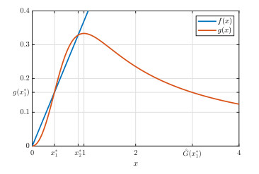
We focus now on the case where g is non-monotone. Suppose that there exists ˆG(x) such that ˆG(x)=ˆg−1og(x), where ˆg(.) denotes the restriction of g to the interval [M,∞). Then, ˆG(x)=x for x∈[M,∞) and ˆG(x)>M>x for x∈[0,M).
Lemma 3.2. Assume that (T1)–(T4) hold. For a given ϕ∈C[x∗1,ˆG(x∗1)]∖{x∗1}, let x be the solution of problem (1.1). Then, the following assertions hold:
(i) if x∗2<M, then x∗1<x(t)<ˆG(x∗1) for all t>0.
(ii) if x∗2≥M and f(ˆG(x∗1))>g(M), then x∗1<x(t)<ˆG(x∗1) for all t>0.
Proof. Without loss of generality, suppose that x∗1<ϕ(0)≤ˆG(x∗1). First, observe that, for a given ϕ∈C[x∗1,ˆG(x∗1)]∖{x∗1}, we have f(ˆG(x∗1))>f(x∗1)=g(x∗1)=g(ˆG(x∗1)), and thus, there exists ϵ>0 such that f(ˆG(x∗1))−ϵ>g(ˆG(x∗1)). We begin by proving that x∗1≤x(t)≤ˆG(x∗1) for all t>0. To this end, in view of Lemma 2.3, we only need to prove that x∗1<xϵ(t):=xϵ(t;ϕ)≤ˆG(x∗1) for all t>0, where xϵ(t):=xϵ(t;ϕ) is the solution of problem (1.1) when replacing f by f−ϵ. Let yϵ:=yϵ(ϕ) be the solution of
| {y′ϵ(t)=−f(yϵ(t))+ϵ+∫τ0h(a)g+(yϵ(t−a))da,t>0,yϵ(t)=ϕ(t),−τ≤t≤0. | (3.1) |
with g+(s)=maxσ∈[0,s]g(σ). Since f is an increasing function, we have f(ˆG(x∗1))−ϵ>g+(ˆG(x∗1)). Accordingly, the function ˆG(x∗1) is a super-solution of problem (3.1). Finally, in view of Theorem 2.1, we obtain xϵ(t)≤yϵ(t)≤ˆG(x∗1) for all t≥0.
We now prove that xϵ(t)>x∗1. Suppose, on the contrary, that there exists t1>0 such that xϵ(t1)=x∗1, xϵ(t)≥x∗1 for all t≤t1, and thus, x′ϵ(t1)≤0. Then, the equation of xϵ(t1) satisfies
| x′ϵ(t1)=−f(xϵ(t1))+ϵ+∫τ0h(a)g(xϵ(t1−a))da>−f(x∗1)+g(x∗1)=0, |
since g(s)≥g(x∗1) for all s∈[x∗1,ˆG(x∗1)]. This reaches a contradiction. Further, from Lemma 2.3, we obtain x(t)≥x∗1. The claim is proved.
Next, let X(t)=x(t)−x∗1. Since f(x∗1)=g(x∗1), the equation of X(t) satisfies
| X′(t)=f(x∗1)−f(x(t))+∫τ0h(a)(g(x(t−a))−g(x∗1))da. |
We know that g(s)≥g(x∗1) for all s∈[x∗1,ˆG(x∗1)]. We then have
| X′(t)≥−LX(t), |
where L is the Lipschitz constant of f. Consequently x(t)>x∗1 for all t>0.
Next, we prove that x(t)<ˆG(x∗1) for all t>0. Suppose, on the contrary, that there exists t1>0 such that x(t1)=ˆG(x∗1), x(t)≤ˆG(x∗1) for all t≤t1 and x′(t1)≥0. Then
| 0≤x′(t1)=−f(x(t1))+∫τ0h(a)g(x(t1−a))da,≤−f(ˆG(x∗1))+g(M). | (3.2) |
Since f is an increasing function and ˆG(x∗1)>M, we have
| 0≤x′(t1)≤−f(M)+g(M). | (3.3) |
Now, the assertion x∗2<M implies that g(M)<f(M), which leads to a contradiction.
When x∗2≥M, inequality (3.2) gives a contradiction by hypothesis. The Lemma is proved.
Using Lemma 3.2, we next prove the following lemma.
Lemma 3.3. Suppose that ϕ∈C[x∗1,ˆG(x∗1)]∖{x∗1}. Assume also that (T1)–(T4) hold. Let x be the solution of problem (1.1). Then, we have
| lim inft→∞x(t)>x∗1, |
provided that one of the following assertions holds:
(i) x∗2<M.
(ii) x∗2≥M and f(ˆG(x∗1))>g(M).
Proof. Firstly, from Lemma 3.2, both assertions imply that x∗1<x(t)<ˆG(x∗1) for all t≥0. Next, observe that there exists ϵ>0 such that
| g(s)>f(x∗1+ϵ)for alls∈[x∗1+ϵ,θϵ], |
with θϵ∈(M,ˆG(x∗1)) and g(θϵ)=g(x∗1+ϵ). Indeed, in view of (T3), minσ∈[x∗1+ϵ,θϵ]g(σ)=g(θϵ)=g(x∗1+ϵ) and from (T4), we have g(x∗1+ϵ)>f(x∗1+ϵ).
Now, consider the following nondecreasing function:
| g_(s)={g(s),for 0<s<ˉm,f(x∗1+ϵ),for ˉm<s<ˆG(x∗1), | (3.4) |
where x∗1<ˉm<x∗1+ϵ, which is a constant satisfying g(ˉm)=f(x∗1+ϵ). From (T2) and (T4), we get g_(s)>f(s) for x∗1<s<x∗1+ϵ and g_(s)<f(s) for s>x∗1+ϵ. Let y(ϕ) be the solution of problem (1.1) when replacing g by g_. Then, according to Theorem 2.1, we have y(t;ϕ)≤x(t;ϕ). In addition, using Theorem 3.1, we obtain
| x∗1<limt→∞y(t;ϕ)=x∗1+ϵ≤lim inft→∞x(t;ϕ). |
The lemma is proved.
Under Lemma 3.3, we prove the following theorem on the global asymptotic stability of the positive equilibrium x∗2<M.
Theorem 3.4. Suppose that ϕ∈C[x∗1,ˆG(x∗1)]∖{x∗1} and x∗2<M. Assume also that (T1)–(T4) hold. Then, the positive equilibrium x∗2 is globally asymptotically stable.
Proof. We first claim that there exists T>0 such that x(t)≤M for all t≥T. Indeed, let xϵ:=xϵ(ϕ) be the solution of problem (1.1) when replacing f by f+ϵ. First, suppose that there exists T>0 such that xϵ(t)≥M for all t≥T. So, since x∗2<M, we have from (T4) that g(M)<f(M). Combining this with (T2), the equation of xϵ satisfies
| x′ϵ(t)≤−f(M)−ϵ+g(M)≤−ϵ, |
which contradicts with xϵ(t)≥M. Hence there exists T>0 such that xϵ(T)<M. We show that xϵ(t)<M for all t≥T. In fact, at the contrary, if there exists t1>T such that xϵ(t1)=M and so x′ϵ(t1)≥0 then,
| x′ϵ(t1)=−f(M)−ϵ+g(M)<0, |
which is a contradiction. Further, according to Lemma 2.3, there exists T>0 such that x(t)≤M for all t≥T and the claim is proved. Finally, since g is a nondecreasing function over (0,M), the global asymptotic stability of x∗2 is proved by applying Theorem 3.1.
Remark 3.5. In the case where g(s)>g(x∗1) for all s>x∗1, the above theorem holds true. In fact, it suffices to replace ˆG(x∗1) in C[x∗1,ˆG(x∗1)]∖{x∗1} by sups∈[−τ,0]ϕ(s).
We focus now on the case where x∗2≥M. To this end, suppose that there exists a unique constant A such that
| A≥M and g(A)=f(M). | (3.5) |
Lemma 3.6. Assume that (T1)–(T4) hold. Suppose also that x∗2≥M and f(A)≥g(M). For a given ϕ∈C[x∗1,ˆG(x∗1)]∖{x∗1} and the solution x:=x(ϕ) of problem (1.1), there exists T>0 such that
| M≤x(t)≤A for all t≥T. |
Proof. We begin by claiming that x∗2≤A. On the contrary, suppose that x∗2>A≥M. Then, due to (T2) and (T3), we have g(x∗2)<g(A)=f(M)<f(x∗2)=g(x∗2), which is a contradiction. The claim is proved.
Next, for a given ϕ∈C[x∗1,ˆG(x∗1)]∖{x∗1}, let xϵ:=xϵ(ϕ) be the solution of problem (1.1) when replacing f by f+ϵ. Since xϵ converges to x as ϵ tends to zero, we only need to prove that there exists T>0 such that xϵ(t)<A for all t≥T. To this end, let yϵ:=yϵ(ϕ) be the solution of problem (1.1), when replacing f by f+ϵ and g by g+ with g+(s)=maxσ∈[0,s]g(σ). By Theorem 2.1, we have xϵ(t)≤yϵ(t) for all t≥0, and thus, we only need to show that yϵ(t)<A for all t≥T. On the contrary, we suppose that yϵ(t)≥A for all t>0. Then, combining the equation of yϵ and the fact that g+(s)=g(M) for all s≥M, we obtain
| y′ϵ(t)≤g(M)−f(A)−ϵ<0, |
which is a contradiction. Then, there exists T>0 such that yϵ(T)<A. We further claim that yϵ(t)<A for all t≥T. Otherwise, there exists t1>T such that yϵ(t1)=A and y′ϵ(t1)≥0. Substituting yϵ(t1) in Eq (1.1), we get
| 0≤y′ϵ(t1)=−f(yϵ(t1))−ϵ+∫τ0h(a)g+(yϵ(t1−a))da,<−f(A)+g(M)≤0, |
which is a contradiction. Consequently, by passing to the limit in ϵ, we obtain that x(t)≤A for all t≥T.
We focus now on the lower bound of x. First, define the function
| g_(s)={g(s),for 0<s<ˉm,f(M),for ˉm<s≤A, | (3.6) |
where x_1^{*} < \bar{m} < M , which is the constant satisfying g(\bar{m}) = f(M) . Note that, due to (T2)–(T4) and condition (3.5), the function \underline{g} is nondecreasing over (0, A) and satisfies
| \begin{equation*} \left \{ \begin{array}{lll} \underline{g}(s)\leq g(s), \quad 0\leq s\leq A,\\ \underline{g}(s) \gt f(s),\quad x^{*}_1 \lt s \lt M,\\ \underline{g}(s) \lt f(s),\quad M \lt s\leq A. \end{array} \right. \end{equation*} |
Let y(\phi) be the solution of problem (1.1) when replacing g by \underline{g} . From Theorem 2.1, we have y(t; \phi)\leq x(t; \phi) for all t > 0 , and from Theorem 3.1, we have \lim\limits_{t\rightarrow \infty}y(t; \phi) = M . Consequently, \liminf\limits_{t\rightarrow \infty}x(t)\geq M . In addition, if, for all T > 0 , there exists (t_n)_n such that t_n > T, y(t_n) = M, \bar{m} < y(s)\leq A for all 0 < s\leq t_n and y'(t_n) < 0 , then, for t_n > T+\tau ,
| \begin{equation*} y'(t_n) = -f(M)+f(M) = 0, \end{equation*} |
which is a contradiction. The lemma is established.
Denote \bar{f} = f|_{[M, A]} the restriction function of f over [M, A] and G(s): = \bar{f}^{-1}(g(s)) for s\in[M, A] . Now, we are ready to state our main theorem related to x^{*}_2\geq M .
Theorem 3.7. Under the assumptions of Lemma 3.6, the positive equilibrium x_2^{*} of problem (1.1) is globally asymptotically stable, provided that one of the following conditions holds:
(H1) fg is a nondecreasing function on [M, A] .
(H2) f+g is a nondecreasing function over [M, A] .
(H3) \dfrac{(GoG)(s)}{s} is a nonincreasing function over [M, x_2^*],
(H4) \dfrac{(GoG)(s)}{s} is a nonincreasing function over [x_2^*, A],
Proof. Denote x_{\infty}: = \liminf_{t\rightarrow \infty}x(t) and x^{\infty}: = \limsup_{t\rightarrow \infty}x(t) . First, suppose that either x^{\infty}\leq x_2^{*} or x_{\infty}\geq x_2^{*} . For x^{\infty}\leq x_2^{*} , we introduce the following function:
| \begin{equation*} \underline{g}(s) = \left\{ \begin{array}{lll} \min\limits_{\sigma\in [s,x_2^{*}]} g(\sigma)&\quad \mbox{for} &\quad x^{*}_1 \lt s \lt x_2^{*},\\ g(x_2^{*}) &\quad \mbox{for} &\quad x_2^{*}\leq s\leq A. \end{array} \right. \end{equation*} |
Let y(\phi) be the solution of problem (1.1) when replacing g by \underline{g}. Since \underline{g}(s)\leq g(s) for all x_1^{*}\leq s\leq x_2^{*} , we have y(t)\leq x(t) for all t > 0. Further, in view of Theorem 3.1, we obtain
| \lim\limits_{t\rightarrow\infty}y(t) = x_2^{*}\leq \limsup\limits_{t \to \infty} x(t) = x^{\infty}\leq x_2^{*}. |
The local stability is obtained by using the same idea as in the proof of Theorem 2.6 in [31].
Now, for x_{\infty}\geq x_2^{*} , we introduce the function
| \begin{equation} \bar{g}(s) = \left\{ \begin{array}{lll} \min\limits_{\sigma\in [s,x_2^{*}]} g(\sigma)&\quad \mbox{for} &\quad x_1^{*} \lt s\leq x_2^{*},\\ \max\limits_{\sigma\in [x_2^{*},s]} g(\sigma)&\quad \mbox{for} &\quad x_2^{*} \lt s\leq A, \end{array} \right. \end{equation} | (3.7) |
and let y(\phi) be the solution of problem (1.1) when replacing g by \bar{g}. As above, we have x(t)\leq y(t) for all t > 0 and y(t) converges to x_2^{*} as t goes to infinity. Next, we suppose that x_{\infty} < x_2^{*} < x^{\infty} and we prove that it is impossible. Indeed, according to Lemma 3.6, we know that, for every solution x of problem (1.1), we have M\leq x_{\infty}\leq x^{\infty}\leq A .
Now, using the fluctuation method (see [28,32]), there exist two sequences t_n\rightarrow \infty and s_n\rightarrow \infty such that
| \begin{equation*} \lim\limits_{n\rightarrow \infty}x(t_n) = x^{\infty}, \;\;\ x'(t_n) = 0, \;\ \forall n\geq 1, \end{equation*} |
and
| \begin{equation*} \lim\limits_{n\rightarrow \infty}x(s_n) = x_{\infty}, \;\;\ x'(s_n) = 0, \;\ \forall n\geq 1. \end{equation*} |
Substituting x(t_n) in problem (1.1), it follows that
| \begin{eqnarray} 0 = -f(x(t_n))+\int_0^{\tau}h(a)g(x(t_n-a))da. \end{eqnarray} | (3.8) |
Since g is nonincreasing over [M, A] , we obtain, by passing to the limit in Eq (3.8), that
| \begin{equation} f(x^{\infty}) \leq g(x_{\infty}). \end{equation} | (3.9) |
Similarly, we obtain
| \begin{equation} f(x_{\infty}) \geq g(x^{\infty}). \end{equation} | (3.10) |
Multiplying the expression (3.9) by g(x^{\infty}) and combining with inequality (3.10), we get
| \begin{equation*} f(x^{\infty})g(x^{\infty}) \leq f(x_{\infty})g(x_{\infty}). \end{equation*} |
This fact, together with the hypothesis (H1) , gives x^{\infty}\leq x_{\infty} , which is a contradiction. In a similar way, we can conclude the contradiction for (H2) . Now, suppose that (H3) holds. First, notice that G makes sense, that is, for all s\in[M, A] , the range of g is contained in [\bar{f}(M), \bar{f}(A)] since \bar{f} is strictly increasing over [M, A]. In fact, for all s\in[M, A] and since g is non-increasing over [M, A] , we have g(A)\leq g(s)\leq g(M). Now, using the fact that f(A)\geq f(M) , we show that
| \begin{equation*} \bar{f}(M)\leq g(s)\leq \bar{f}(A) \quad \mbox{for all} \;\; s\in [M,A]. \end{equation*} |
Therefore, the function G is nonincreasing and maps [M, A] to [M, A] . In view of inequalities (3.9) and (3.10) and the monotonicity of \bar{f} , we arrive at
| \begin{equation} x^{\infty} \leq G(x_{\infty}), \end{equation} | (3.11) |
and
| \begin{equation} x_{\infty} \geq G(x^{\infty}), \end{equation} | (3.12) |
with G(s) = \bar{f}^{-1}(g(s)). Now, applying the function G to inequalities (3.11) and (3.12), we find
| \begin{equation*} x_{\infty} \geq G(x^{\infty}) \geq (GoG)(x_{\infty}), \end{equation*} |
which gives
| \begin{equation} \dfrac{(GoG)(x_{\infty})}{x_{\infty}}\leq 1 = \dfrac{(GoG)(x_2^{*})}{x_2^{*}}. \end{equation} | (3.13) |
Due to (H3) , it ensures that x_2^{*}\leq x_{\infty} , which is impossible. Using the same arguments as above, we obtain a contradiction for (H4). The theorem is proved.
Remark 3.8. In the case where g(s) > g(A) for all s > M, the two above results hold true. In fact, it suffices to replace A in Lemma 3.6 and Theorem 3.7 by B defined in (T1).
For the tangential case where two positive equilibria x^{*}_1 and x^{*}_2 are equal, we have the following theorem
Theorem 3.9. Suppose that (T1)–(T3) hold. Suppose that, in addition to the trivial equilibrium, problem (1.1) has a unique positive equilibrium x^{*}_1 . Then
(i) for \phi\in C_{+}, there exists T > 0 such that 0\leq x(t)\leq M for all t\geq T.
(ii) \phi\in C_{[x^{*}_1, \hat{G}(x_1^{*})]}\setminus\{x_1^{*}\} implies that x^{*}_1 < x(t)\leq M for all t\geq T.
(iii) if \phi\in C_{[x^{*}_1, \hat{G}(x_1^{*})]} , then x^{*}_1 attracts every solution of problem (1.1) and x^{*}_1 is unstable.
Proof. The uniqueness of the positive equilibrium implies that x^{*}_1\leq M and g(x) < f(x) for all x\neq x^{*}_1 . For (ⅰ), suppose that there exists t_0 > 0 such that x(t)\geq M for all t\geq t_0. Then, by substituting x in Eq (1.1), we get
| \begin{equation*} x'(t)\leq -f(M)+g(M) \lt 0. \end{equation*} |
This is impossible and then there exists T > 0 such that x(T) < M . Next, if there exists t_1 > T such that x(t_1) = M and x(t)\leq M for all t\leq t_1 , then
| \begin{equation*} 0\leq x'(t_1)\leq -f(M)+g(M) \lt 0. \end{equation*} |
Consequently (ⅰ) holds. We argue as in the proof of Lemma 3.2 (ⅰ), to show (ⅱ). Concerning (ⅲ), we consider the following Lyapunov functional
| \begin{equation*} \begin{array}{lll} V(\phi)& = & \int_{x^{*}_1}^{\phi(0)}(g(s)-g(x_1^{*}))ds+\dfrac{1}{2} \int_0^{\tau}\psi(a)(g(\phi(-a))-g(x_1^{*}))^2da, \end{array} \end{equation*} |
where \psi(a) = \int_{a}^{\tau}h(\sigma)d\sigma . As in the proof of Theorem 3.1, the derivative of V along the solution of problem (1.1) gives
| \begin{array}{lll} \dfrac{dV({x}_{t})}{dt} = -\dfrac{1}{2} \int_{0}^{\tau}h(a)\big[ g(x(t))-g(x(t-a))\big]^2da+\big[g(x(t))-g(x^{*}_1)\big] \big[ g(x(t))-f(x(t))\big], \quad \forall t \gt 0. \end{array} |
Since g(s) < f(s) for all s\neq x^{*}_1 and g(s)\geq g(x^{*}_1) for all s\in [x^{*}_1, M] , we have dV(x_t)/dt \leq 0 . By LaSalle invariance theorem, x^{*}_1 attracts every solution x(\phi) of problem (1.1) with \phi \in C_{[x^{*}_1, \hat{G}(x_1^{*})]}. From Theorems 2.5 and 3.4, we easily show that x_1 is unstable.
In this section, we apply our results to the following distributed delay differential equation:
| \begin{equation} x'(t) = -\mu x(t)+ \int_0^{\tau}h(a)\dfrac{kx^{2}(t-a)}{1+2x^3(t-a)}da, \;\ \mbox{for} \;\ t\geq 0, \end{equation} | (4.1) |
where \mu, k are positive constants. The variable x(t) stands for the maturated population at time t and \tau > 0 is the maximal maturation time of the species under consideration. h(a) is the maturity rate at age a . In this model, the death function f(x) = \mu x and the birth function g(x) = kx^{2}/(1+2x^3) reflect the so called Allee effect. Obviously, the functions f and g satisfy the assumptions (T1)–(T3) and g reaches the maximum value k/3 at the point M = 1. The equilibria of Eq (4.1) satisfies the following equation:
| \begin{equation} \mu x = \dfrac{kx^{2}}{1+2x^3}. \end{equation} | (4.2) |
Analyzing Eq (4.2), we obtain the following proposition.
Proposition 4.1. Equation (4.1) has a trivial equilibrium x = 0 . In addition
(i) if \mu > \dfrac{2^{\frac{1}{3}}}{3}k , then Eq (4.1) has no positive equilibrium;
(ii) if \mu = \dfrac{2^{\frac{1}{3}}}{3}k , then Eq (4.1) has exactly one positive equilibrium x_1^{*} ;
(iii) if 0 < \mu < \dfrac{2^{\frac{1}{3}}}{3}k , then Eq (4.1) has exactly two positive equilibria x^{*}_1 < x^{*}_2 . Moreover,
(iii)-a if \dfrac{k}{3} < \mu < \dfrac{2^{\frac{1}{3}}}{3}k, then 0 < x^{*}_1 < x_2^{*} < 1;
(iii)-b if 0 < \mu\leq \dfrac{k}{3}, then 0 < x^{*}_1 < 1\leq x^{*}_2.
Using Theorem 2.6, we obtain
Theorem 4.2. If \mu > \dfrac{2^{\frac{1}{3}}}{3}k, then the trivial equilibrium of Eq (4.1) is globally asymptotically stable for all \phi \in C_{+}.
For the case (ⅲ)-a in Proposition 4.1 we have the following result
Theorem 4.3. Suppose that \dfrac{k}{3} < \mu < \dfrac{2^{\frac{1}{3}}}{3}k. Then
(i) The trivial equilibrium of Eq (4.1) is globally asymptotically stable for all \phi \in C_{[0, x^{*}_1]}\setminus\{x^{*}_1\}.
(ii) The positive equilibrium x_1^{*} is unstable and the positive equilibrium x^{*}_2 is globally asymptotically stable for all \phi \in C_{[x^{*}_1, \hat{G}(x^{*}_1)]}\setminus\{x^{*}_1\} , where \hat{G}(x^{*}_1)\in [1, \infty) satisfies g(\hat{G}(x^{*}_1)) = g(x^{*}_1).
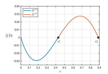
(iii) There exists two heteroclinic orbits X^{(1)} and X^{(2)} connecting 0 to x^{*}_1 and x^{*}_1 to x^{*}_2 , respectively.
Proof. (ⅰ) and (ⅱ) directly follow from Proposition 4.1, (ⅲ)-a and Theorems 2.5 and 3.4.
For (ⅲ), we follow the same proof as in Theorem 4.2 in [5]. See also [18]. For the sake of completeness, we rewrite it. Let K = \{x^{*}_1\}. Clearly, K is an isolated and unstable compact invariant set in C_{[0, x^{*}_1]} and C_{[x^{*}_1, \hat{G}(x^{*}_1)]}.
By applying Corollary 2.9 in [33] to \Phi_{|{\bf{R}}^{+}\times C[0, x^{*}_1]} and \Phi_{|{\bf{R}}^{+}\times C[x^{*}_1, \hat{G}(x^{*}_1)]}, respectively, there exist two pre-compact full orbits X^{(1)}:{\bf{R}}\rightarrow C_{[0, x^{*}_1]}\setminus\{0\} and X^{(2)}:{\bf{R}}\rightarrow C_{[x^{*}_1, \hat{G}(x^{*}_1)]}\setminus\{0\} such that \alpha(X^{1}) = \alpha(X^{2}) = K. This together with statements (i) and (ii) gives \omega{(X^{(1)})} = \{0\} and \omega{(X^{(2)})} = \{x^{*}_2\} . In other words, there exist two heteroclinic orbits X^{(1)} and X^{(2)} , which connect 0 to x^{*}_1 and x^{*}_1 to x^{*}_2 , respectively. This completes the proof.
For the case (ⅲ)-b in Proposition 4.1, we first show that
| \begin{equation} f(A)\geq g(M) \;\ \mbox{with} \;\ g(A) = f(M)\;\ \mbox{and} \;\ A\geq M. \end{equation} | (4.3) |
Lemma 4.4. Suppose that f(s) = \mu s . Condition (4.3) holds if and only if M\leq \dfrac{1}{\mu}g(\dfrac{1}{\mu}g(M)).
Proof. It follows that f(A)\geq g(M) if and only if A\geq f^{-1}(g(M))\geq M . Since g is a decreasing function over [M, \infty) , we have g(A)\leq g(f^{-1}(g(M))) = g(\dfrac{1}{\mu}(g(M))) . Moreover, since g(A) = f(M) , we have M\leq \dfrac{1}{\mu}g(\dfrac{1}{\mu}g(M)) . The lemma is proved.
Lemma 4.5. For Eq (4.1), condition (4.3) holds if and only if
| \begin{equation} 0 \lt \mu\leq \dfrac{k}{3}. \end{equation} | (4.4) |
Proof. By a straightforward computation, we have f^{-1}(x) = x/\mu . For G(x) = g(x)/\mu , we obtain
| \begin{equation*} (GoG)(x) = \dfrac{x(2px^{6}+px^{3})}{8x^{9}+(12+2p)x^{6}+6x^{3}+1}, \end{equation*} |
where p = k^{3}/\mu^{3}. By applying Lemma 4.4, it is readily to see that 1\leq (GoG)(1) holds if and only if
| \begin{equation*} 1\leq \dfrac{3p}{2p+27}, \end{equation*} |
and thus, 0 < \mu\leq k/3.
Theorem 4.6. Suppose that 0 < \mu \leq \dfrac{k}{3}. Then, the positive equilibrium x^{*}_2 of Eq (4.1) is globally asymptotically stable for all \phi \in C_{[x^{*}_1, \hat{G}(x^{*}_1)]}\setminus\{x^{*}_1\} , where \hat{G}(x^{*}_1)\in [1, \infty) satisfies g(\hat{G}(x^{*}_1)) = g(x^{*}_1).
Proof. Observe that, in view of Lemmas 4.4 and 4.5, all hypotheses of Lemma 3.6 are satisfied. Now, in order to apply Theorem 3.7, we only show that \dfrac{(GoG)(x)}{x} is nonincreasing over [M, A]. Indeed, by a simple computation, we have
| \begin{equation*} \bigg(\dfrac{(GoG)(x)}{x}\bigg)' = \dfrac{-48px^{14}-48px^{11}-6p^{2}x^{8}+12px^{5}+3px^{2}}{[8x^{9}+(12+2p)x^{6}+6x^{3}+1]^{2}}, \end{equation*} |
where p = k^{3}/\mu^{3}. Finally, observe that
| \begin{equation*} \bigg(\dfrac{(GoG)(x)}{x}\bigg)' \lt 0, \end{equation*} |
for x\geq 1. In this case, both of (H3) and (H4) in Theorem 3.7 hold. This completes the proof.
Finally, for the tangential case, we have
Theorem 4.7. Suppose that \mu = \dfrac{2^{\frac{1}{3}}}{3}k. Then
(i) The trivial equilibrium of Eq (4.1) is globally asymptotically stable for all \phi \in C_{[0, x^{*}_1]}\setminus\{x^{*}_1\}.
(ii) If \phi \in C_{[x^{*}_1, \hat{G}(x^{*}_1)]}\setminus\{x^{*}_1\} , then the unique positive equilibrium x_1^{*} is unstable and attracts every solution of Eq (4.1).
Proof. The proof of this theorem follows immediately from Theorems 2.5 and 3.9.
In this section, we perform numerical simulation that supports our theoretical results. As in Section 4, we assume that
| f(x) = \mu x, \quad g(x) = \frac{kx^2}{1+2x^3}, |
and confirm the validity of Theorems 4.2, 4.3, 4.6 and 4.7. In what follows, we fix
| \begin{equation} \tau = 1, \quad k = 1, \quad h(a) = \frac{e^{-(a-0.5\tau)^2 \times 10^{2}}}{\int_0^\tau e^{-(\sigma-0.5\tau)^2 \times 10^{2}} d\sigma} \end{equation} | (5.1) |
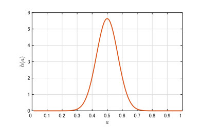
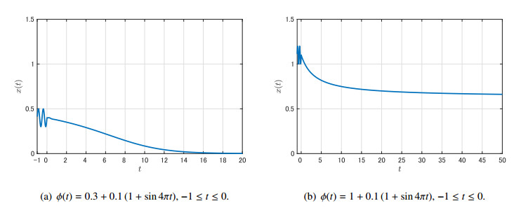
and change \mu and \phi . Note that \frac{2^{\frac{1}{3}}}{3}k \approx 0.42 and h is a Gaussian-like distribution as shown in Figure 1.
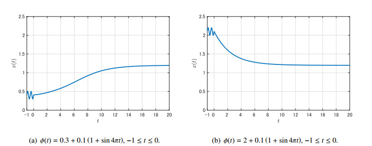
First, let \mu = 0.5 . In this case, \mu > \dfrac{2^{\frac{1}{3}}}{3} k and thus, by Theorem 4.2, the trivial equilibrium is globally asymptotically stable. In fact, Figure 2 shows that x(t) converges to 0 as t increases for different initial data.
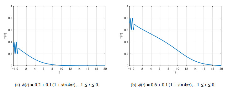
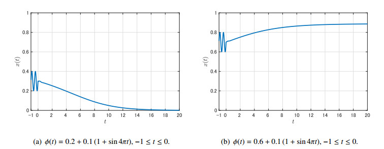
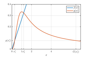
Next, let \mu = 0.37 . In this case, \dfrac{k}{3} < \mu < \dfrac{2^{\frac{1}{3}}}{3}k and x_1^* \approx 0.43 , x_2^* \approx 0.89 and \hat{G}(x_1^*) \approx 3.09 (Figure 3). Hence, by Theorem 4.3, we see that the trivial equilibrium is globally asymptotically stable for \phi \in C_{[0, x_1^*]} \setminus \{ x_1^* \} , whereas the positive equilibrium x_2^* is so for \phi \in C_{[x_1^*, \hat{G}(x_1^*)]} \setminus \{ x_1^* \} . In fact, Figure 4 shows such a bistable situation. Moreover, heteroclinic orbits X^{(1)} and X^{(2)} , which were stated in Theorem 4.3 (ⅲ), are shown in Figure 5.
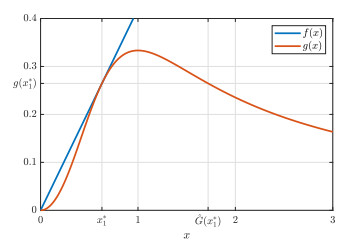
Thirdly, let \mu = 0.27 < \dfrac{k}{3} \approx 0.33 . In this case, we have x_1^* \approx 0.28 , x_2^* \approx 1.2 and \hat{G}(x_1^*) \approx 6.52 (Figure 6). Thus, by Theorem 4.6, we see that the positive equilibrium x_2^* is globally asymptotically stable for \phi \in C_{[x_1^*, \hat{G}(x_1^*)]} \setminus \{ x_1^* \} . In fact, Figure 7 shows that x(t) converges to x_2^* as t increases for different initial data.
Finally, let \mu = \dfrac{2^{\frac{1}{3}}}{3}k \approx 0.42 . In this case, we have x_1^* \approx 0.63 and \hat{G}(x_1^*) \approx 1.72 (Figure 8). By Theorem 4.7, we see that the trivial equilibrium is globally asymptotically stable for \phi \in C_{[0, x_1^*]} \setminus \{ x_1^* \} , whereas x_1^* is unstable and attracts all solutions for \phi \in C_{[x_1^*, \hat{G}(x_1^*)]} \setminus \{ x_1^* \} . In fact, Figure 9 shows such two situations.
In this paper, we studied the bistable nonlinearity problem for a general class of functional differential equations with distributed delay, which includes many mathematical models in biology and ecology. In contrast to the previous work [5], we considered both cases x_2^* < M and x_2^* \geq M , and obtained sufficient conditions for the global asymptotic stability of each equilibrium. The general results were applied to a model with Allee effect in Section 4, and numerical simulation was performed in Section 5. It should be pointed out that our theoretical results are robust for the variation of the form of the distribution function h . This might suggest us that the distributed delay is not essential for the dynamical system of our model. We conjecture that our results still hold for \tau = \infty , and we leave it for a future study. Extension of our results to a reaction-diffusion equation could also be an interesting future problem.
We deeply appreciate the editor and the anonymous reviewers for their helpful comments to the earlier version of our manuscript. The first author is partially supported by the JSPS Grant-in-Aid for Early-Career Scientists (No.19K14594). The second author is partially supported by the DGRSDT, ALGERIA.
All authors declare no conflicts of interest in this paper.
| [1] | C. Berge, Graphs and Hypergraphs, 2nd ed., North-Holland, Amsterdam, 1976. |
| [2] |
L. Boxer, A classical construction for the digital fundamental group, J. Math. Imaging Vis., 10 (1999), 51–62. doi: 10.1023/A:1008370600456

|
| [3] | S.-E. Han, Non-product property of the digital fundamental group, Information Sciences 171(1-3) (2005) 73-91. |
| [4] | S.-E. Han, On the simplicial complex stemmed from a digital graph, Honam Mathematical Journal, 27 (2005), 115–129. |
| [5] |
S.-E. Han, An equivalent property of a normal adjacency of a digital product, Honam Mathematical Journal, 36 (2014), 199–215. doi: 10.5831/HMJ.2014.36.1.199
|
| [6] |
S.-E. Han, Compatible adjacency relations for digital products, Filomat, 31 (2017), 2787–2803. doi: 10.2298/FIL1709787H
|
| [7] | S.-E. Han, Estimation of the complexity of a digital image form the viewpoint of fixed point theory, Appl. Math. Comput. 347 (2019), 236–248. |
| [8] |
S.-E. Han, Digital k-contractibility of an n-times iterated connected sum of simple closed k-surfaces and almost fixed point property, Mathematics, 8 (2020), 345. doi: 10.3390/math8030345
|
| [9] |
G. T. Herman, Oriented surfaces in digital spaces, CVGIP: Graphical Models and Image Processing, 55 (1993), 381–396. doi: 10.1006/cgip.1993.1029
|
| [10] | J.-M. Kang, S.-E. Han, The product property of the almost fixed point property, AIMS Math. 6 (2021), 7215–7228. |
| [11] | T. Y. Kong, A. Rosenfeld, Topological Algorithms for the Digital Image Processing, Elsevier Science, Amsterdam, 1996. |
| [12] | A. Rosenfeld, Digital topology, Amer. Math. Monthly, 86 (1979), 76–87. |
| [13] |
A. Rosenfeld, Continuous functions on digital pictures, Pattern Recogn. Lett., 4 (1986), 177–184. doi: 10.1016/0167-8655(86)90017-6
|
| 1. | Soufiane Bentout, Sunil Kumar, Salih Djilali, Hopf bifurcation analysis in an age-structured heroin model, 2021, 136, 2190-5444, 10.1140/epjp/s13360-021-01167-8 | |
| 2. | Salih Djilali, Soufiane Bentout, Behzad Ghanbari, Sunil Kumar, Spatial patterns in a vegetation model with internal competition and feedback regulation, 2021, 136, 2190-5444, 10.1140/epjp/s13360-021-01251-z | |
| 3. | Soufiane Bentout, Salih Djilali, Sunil Kumar, Mathematical analysis of the influence of prey escaping from prey herd on three species fractional predator-prey interaction model, 2021, 572, 03784371, 125840, 10.1016/j.physa.2021.125840 | |
| 4. | Salih Djilali, Behzad Ghanbari, Dynamical behavior of two predators–one prey model with generalized functional response and time-fractional derivative, 2021, 2021, 1687-1847, 10.1186/s13662-021-03395-9 | |
| 5. | Fethi Souna, Salih Djilali, Abdelkader Lakmeche, Spatiotemporal behavior in a predator–prey model with herd behavior and cross-diffusion and fear effect, 2021, 136, 2190-5444, 10.1140/epjp/s13360-021-01489-7 | |
| 6. | Mohammed Nor Frioui, Tarik Mohammed Touaoula, 2023, 9780323995573, 1, 10.1016/B978-0-32-399557-3.00006-5 | |
| 7. | Soufiane Bentout, Salih Djilali, Sunil Kumar, Tarik Mohammed Touaoula, Threshold dynamics of difference equations for SEIR model with nonlinear incidence function and infinite delay, 2021, 136, 2190-5444, 10.1140/epjp/s13360-021-01466-0 | |
| 8. | Toshikazu Kuniya, Tarik Mohammed Touaoula, Global dynamics for a class of reaction–diffusion equations with distributed delay and non-monotone bistable nonlinearity, 2022, 0003-6811, 1, 10.1080/00036811.2022.2102488 |


Figures(4)

Jeong Min Kang, Sang-Eon Han, Sik Lee. Digital products with PN_k -adjacencies and the almost fixed point property in DTC_k^\blacktriangle [J]. AIMS Mathematics, 2021, 6(10): 11550-11567. doi: 10.3934/math.2021670

 DownLoad:
