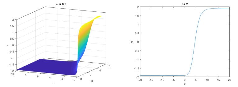
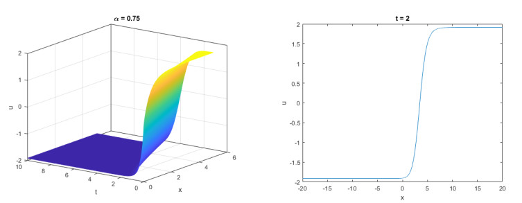
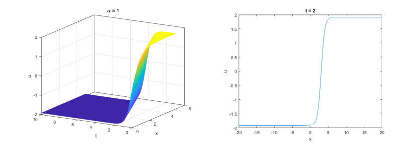
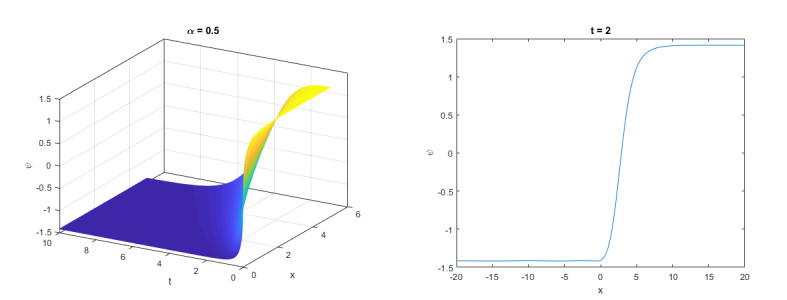
We construct new solitary structures for time fractional Phi-4 and space-time fractional simplified modified Camassa-Holm (MCH) equations, utilizing the unified solver technique. The time (space-time) fractional derivatives are defined via sense of the new conformable fractional derivative. The unified solver technique extract vital solutions in explicit way. The obtained solutions may be beneficial for explaining many complex phenomena arising in fluid mechanics, nuclear, plasma and particle physics. The unified solver method is a vital tool for handling further models arising in applied science and new physics. For detailed physical dynamical representation of our results, 3D and 2D profiles to some of the gained solutions are also illustrated using Matlab software.
Citation: Mahmoud A. E. Abdelrahman, S. Z. Hassan, R. A. Alomair, D. M. Alsaleh. Fundamental solutions for the conformable time fractional Phi-4 and space-time fractional simplified MCH equations[J]. AIMS Mathematics, 2021, 6(6): 6555-6568. doi: 10.3934/math.2021386
We construct new solitary structures for time fractional Phi-4 and space-time fractional simplified modified Camassa-Holm (MCH) equations, utilizing the unified solver technique. The time (space-time) fractional derivatives are defined via sense of the new conformable fractional derivative. The unified solver technique extract vital solutions in explicit way. The obtained solutions may be beneficial for explaining many complex phenomena arising in fluid mechanics, nuclear, plasma and particle physics. The unified solver method is a vital tool for handling further models arising in applied science and new physics. For detailed physical dynamical representation of our results, 3D and 2D profiles to some of the gained solutions are also illustrated using Matlab software.

| [1] |
M. K. Kaplan, A. E. Bekir, A novel analytical method for time-fractional differential equations, Optik, 127 (2016), 8209–8214. doi: 10.1016/j.ijleo.2016.05.152

|
| [2] | F. Tchier, M. Inc, Z. S. Korpinar, D. Baleanu, Solution of the time fractional reaction-diffusion equations with residual power series method, Adv. Mech. Eng., 8 (2016), 1–10. |
| [3] |
A. Zafar, Rational exponential solutions of conformable spacetime fractional equal width equations, Nonlinear Eng., 8 (2019), 350–355. doi: 10.1515/nleng-2018-0076
|
| [4] |
D. Foukrach, Approximate solution to a Bürgers system with time and space fractional derivatives using Adomian decomposition method, J. Interdisciplinary Math., 21 (2018), 111–125. doi: 10.1080/09720502.2014.986914
|
| [5] |
S. S. Ray, New analytical exact solutions of time fractional kdv-KZK equation by Kudryashov methods, Chinese Phys. B, 25 (2016), 040204. doi: 10.1088/1674-1056/25/4/046105
|
| [6] |
S. Sarwar, S. Iqbal, Stability analysis, dynamical behavior and analytical solutions of nonlinear fractional differential system arising in chemical reaction, Chinese J. Phys., 56 (2018), 374–384. doi: 10.1016/j.cjph.2017.11.009
|
| [7] | K. Hosseini, F. Samadani, D. Kumar, M. Faridi, New optical solitons of cubic-quartic nonlinear Schrzödinger equation, Optik., 157 (2018), 1101–1105. |
| [8] |
Q. Zhou, A. Sonmezoglu, M. Ekici, M. Mirzazadeh, Optical solitons of some fractional differential equations in nonlinear optics, J. Mod. Optic., 64 (2017), 2345–2349. doi: 10.1080/09500340.2017.1357856
|
| [9] |
F. S. Khodadad, F. Nazari, M. Eslami, H. Rezazadeh, Soliton solutions of the conformable fractional Zakharov–Kuznetsov equation with dual-power law nonlinearity, Opt. Quant. Electron., 49 (2017), 1–12. doi: 10.1007/s11082-016-0848-8
|
| [10] |
B. Lu, The first integral method for some time fractional differential equations, J. Math. Anal. Appl., 395 (2012), 684–693. doi: 10.1016/j.jmaa.2012.05.066
|
| [11] |
K. Hosseini, P. Mayeli, R. Ansari, Modified Kudryashov method for solving the conformable time fractional Klein-Gordon equations with quadratic and cubic nonlinearities, Optik, 130 (2017), 737–742. doi: 10.1016/j.ijleo.2016.10.136
|
| [12] | S. Zhang, Q-A. Zong, D. Liu, Q. Gao, A generalized exp-function method for fractional riccati differential equations, Communications in Fractional Calculus, 1 (2010), 48–51. |
| [13] |
M. Younis, S. T. R. Rizvi, Dispersive dark optical soliton in (2+1)-dimensions by $(\frac{G^{'}}{G})$-expansion with dual-power law nonlinearity, Optik, 126 (2015), 5812–5814. doi: 10.1016/j.ijleo.2015.08.233
|
| [14] |
N. Faraz, Y. Khan, H. Jafari, A. Yildirim, M. Madani, Fractional variational iteration method via modified Riemann- Liouville derivative, J. King Saud Univ. Sci., 23 (2011), 413–417. doi: 10.1016/j.jksus.2010.07.025
|
| [15] |
B. Tong, Y. He, L. Wei, X. Zhang, A generalized fractional sub-equation method for fractional differential equations with variable coefficients, Phys. Lett. A, 376 (2012), 2588–2590. doi: 10.1016/j.physleta.2012.07.018
|
| [16] |
S. S. Ray, S. Sahoo, A novel analytical method with fractional complex transform for new exact solutions of time-fractional fifth-order Sawada-Kotera equation, Rep. Math. Phys., 75 (2015), 63–72. doi: 10.1016/S0034-4877(15)60024-6
|
| [17] | I. Podlubny, Fractional differential equations, Academic Press, 1998. |
| [18] |
R. Khalil, M. Al Horani, A. Yousef, M. Sababheh, A new definition of fractional derivative, J. Comput. Appl. Math., 264 (2014), 65–70. doi: 10.1016/j.cam.2014.01.002
|
| [19] |
T. Abdeljawad, On conformable fractional calculus, J. Comput. Appl. Math., 279 (2015), 57–66. doi: 10.1016/j.cam.2014.10.016
|
| [20] |
H. Rezazadeh, H. Tariq, M. Eslami, M. Mirzazadeh, Q. Zhou, New exact solutions of nonlinear conformable time-fractional Phi-4 equation, Chinese J. Phys., 56 (2018), 2805–2816. doi: 10.1016/j.cjph.2018.08.001
|
| [21] |
K. Zeliha, Some analytical solutions by mapping methods for non-linear conformable time-fractional Phi-4 equation, Therm. Sci., 23 (2019), 1815–1822. doi: 10.2298/TSCI190108341K
|
| [22] |
M. M. Khader, S. Kumar, An accurate numerical method for solving the linear fractional Klein-Gordon equation, Math. Method. Appl. Sci., 37 (2014), 2972–2979. doi: 10.1002/mma.3035
|
| [23] |
X. Deng, M. Zhao, X. Li, Travelling wave solutions for a nonlinear variant of the PHI-four equation, Math. Comput. Model., 49 (2009), 617–622. doi: 10.1016/j.mcm.2008.03.011
|
| [24] |
H. Tariq, G. Akram, New approach for exact solutions of time fractional Cahn-Allen equation and time fractional Phi-4 equation, Physica A, 473 (2017), 352–362. doi: 10.1016/j.physa.2016.12.081
|
| [25] |
H. Rezazadeh, K. K. Ali, M. Eslami, M. Mirzazadeh, H. Yépez-Martínez, On the soliton solutions to the space-time fractional simplified MCH equation, J. Interdisciplinary Math., 22 (2019), 149–165. doi: 10.1080/09720502.2019.1597431
|
| [26] | M. Shakeel, Q. M. Ul-Hassan, J. Ahmad, Applications of the novel $(\frac{G^{'}}{G})-$ expansion method for a time fractional simplified modified MCH equation, Abstr. Appl. Anal., 2014 (2014), 601961. |
| [27] |
M. A. E. Abdelrahman, A note on Riccati-Bernoulli sub-ODE method combined with complex transform method applied to fractional differential equations, Nonlinear Engineering Modeling and Application, 7 (2018), 279–285. doi: 10.1515/nleng-2017-0145
|
| [28] |
S. Z. Hassan, M. A. E. Abdelrahman, Solitary wave solutions for some nonlinear time fractional partial differential equations, Pramana, 91 (2018), 1–9. doi: 10.1007/s12043-018-1574-5
|
| [29] |
X. F. Yang, Z. C. Deng, Y. Wei, A Riccati-Bernoulli sub-ODE method for nonlinear partial differential equations and its application, Adv. Differ. Equ, 2015 (2015), 1–17. doi: 10.1186/s13662-014-0331-4
|
| [30] |
S. Sahoo, S. S. Ray, Improved fractional sub-equation method for (3+1)-dimensional generalized fractional KdV-Zakharov-Kuznetsov equations, Comput. Math. Appl., 70 (2015), 158–166. doi: 10.1016/j.camwa.2015.05.002
|
| [31] |
S. Arbabi, M. Najafi, Exact solitary wave solutions of the complex nonlinear Schrödinger equations, Optik, 127 (2016), 4682–4688. doi: 10.1016/j.ijleo.2016.02.008
|
| [32] |
H. Bulut, T. A. Sulaiman, H. M. Baskonus, Dark, bright optical and other solitons with conformable space-time fractional second-order spatiotemporal dispersion, Optik, 163 (2018), 1–7. doi: 10.1016/j.ijleo.2018.02.086
|
| [33] |
M. Inc, A. I. Aliyu, A. Yusuf, D. Baleanu, Soliton solutions and stability analysis for some conformable nonlinear partial differential equations in mathematical physics, Opt. Quant. Electron, 50 (2018), 1–14. doi: 10.1007/s11082-017-1266-2
|
| [34] | T. A. Sulaiman, H. Bulut, H. M. Baskonus, Optical solitons to the fractional perturbed NLSE in nano-fibers, Discrete Cont. Dyn. S, 13 (2020), 925–936. |
| [35] |
M. A. E. Abdelrahman, H. AlKhidhr, Closed-form solutions to the conformable space-time fractional simplified MCH equation and time fractional Phi-4 equation, Results Phys., 18 (2020), 103294. doi: 10.1016/j.rinp.2020.103294
|
| [36] | C. Q. Dai, J. F. Zhang, Jacobian elliptic function method for nonlinear differential difference equations, Chaos Solution. Fract., 27 (2006) 1042–1047. |
| [37] | Q. Wanga, Y. Chen, H. Zhang, An extended Jacobi elliptic function rational expansion method and its application to (2+1)-dimensional dispersive long wave equation, Phys. Lett. A, 289 (2005), 411–426. |
| [38] |
Q. Zhang, X. Li, K. Pan, Y. Ren, Linearized ADI schemes for two-dimensional space-fractional nonlinear Ginzburg–Landau equation, Comput. Math. Appl., 80 (2020), 1201–1220. doi: 10.1016/j.camwa.2020.05.027
|
| [39] |
Q. Zhang, L. Zhang, H. W. Sun, A three-level finite difference method with preconditioning technique for two-dimensional nonlinear fractional complex Ginzburg–Landau equations, J. Comput. Appl. Math., 389 (2021), 113355. doi: 10.1016/j.cam.2020.113355
|
| [40] | Q. Zhang, M. Chen, Y. Xu, D. Xu, Compact $\theta$-method for the generalized delay diffusion equation, Appl. Math. Comput., 316 (2018), 357–369. |
| [41] |
Q. Zhang, T. Li, Asymptotic stability of compact and linear $\theta$-methods for space fractional delay generalized diffusion equation, J. Sci. Comput., 81 (2019), 2413–2446. doi: 10.1007/s10915-019-01091-1
|
| [42] |
V. E. Zakharov, L. A. Ostrovsky, Modulation instability: The beginning, Physica D, 238 (2009), 540–548. doi: 10.1016/j.physd.2008.12.002
|
| [43] |
M. Arshad, A. R. Seadawy, D. Lu, W. Jun, Modulation instability analysis of modify unstable nonlinear Schrödinger dynamical equation and its optical soliton solutions, Results in Phys., 7 (2017), 4153–4161. doi: 10.1016/j.rinp.2017.10.029
|
Figures(6)

Mahmoud A. E. Abdelrahman, S. Z. Hassan, R. A. Alomair, D. M. Alsaleh. Fundamental solutions for the conformable time fractional Phi-4 and space-time fractional simplified MCH equations[J]. AIMS Mathematics, 2021, 6(6): 6555-6568. doi: 10.3934/math.2021386


 DownLoad: