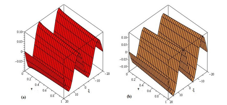
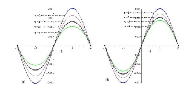
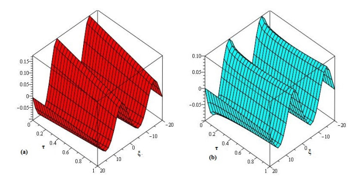
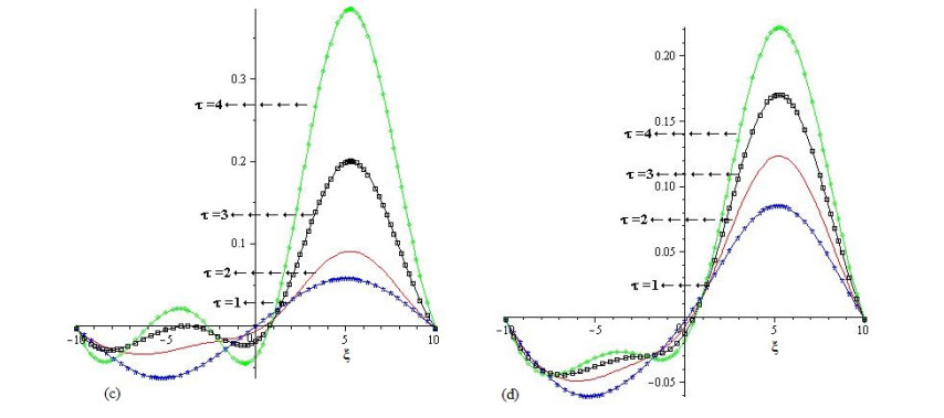
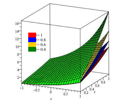
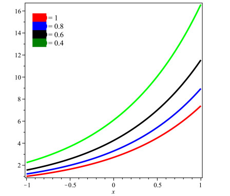
The present research paper is related to the analytical solution of fractional-order nonlinear Swift-Hohenberg equations using an efficient technique. The presented model is related to the temperature and thermal convection of fluid dynamics which can also be used to explain the formation process in liquid surfaces bounded along a horizontally well-conducting boundary. In this work Laplace Adomian decomposition method is implemented because it require small volume of calculations. Unlike the variational iteration method and Homotopy pertubation method, the suggested technique required no variational parameter and having simple calculation of fractional derivative respectively. Numerical examples verify the validity of the suggested method. It is confirmed that the present method's solutions are in close contact with the solutions of other existing methods. It is also investigated through graphs and tables that the suggested method's solutions are almost identical with different analytical methods.
Citation: Jiabin Xu, Hassan Khan, Rasool Shah, A.A. Alderremy, Shaban Aly, Dumitru Baleanu. The analytical analysis of nonlinear fractional-order dynamical models[J]. AIMS Mathematics, 2021, 6(6): 6201-6219. doi: 10.3934/math.2021364
The present research paper is related to the analytical solution of fractional-order nonlinear Swift-Hohenberg equations using an efficient technique. The presented model is related to the temperature and thermal convection of fluid dynamics which can also be used to explain the formation process in liquid surfaces bounded along a horizontally well-conducting boundary. In this work Laplace Adomian decomposition method is implemented because it require small volume of calculations. Unlike the variational iteration method and Homotopy pertubation method, the suggested technique required no variational parameter and having simple calculation of fractional derivative respectively. Numerical examples verify the validity of the suggested method. It is confirmed that the present method's solutions are in close contact with the solutions of other existing methods. It is also investigated through graphs and tables that the suggested method's solutions are almost identical with different analytical methods.

| [1] | K. B. Oldham, J. Spanier, The Fractional Calculus, vol. 111 of Mathematics in science and engineering, 1974. |
| [2] | A. A. A. Kilbas, H. M. Srivastava, J. J. Trujillo, Theory and applications of fractional differential equations, Elsevier Science Limited, 204 (2006). |
| [3] | K. S. Miller, B. Ross, An introduction to the fractional calculus and fractional differential equations, Wiley, 1993. |
| [4] |
M. Caputo, Linear models of dissipation whose Q is almost frequency independent-II, Geophys. J. Int., 13 (1967), 529-539. doi: 10.1111/j.1365-246X.1967.tb02303.x

|
| [5] | F. Yin, J. Song, X. Cao, A general iteration formula of VIM for fractional heat-and wave-like equations, J. Appl. Math., 2013. |
| [6] |
A. S. Arife, S. K. Vanani, F. Soleymani, The Laplace homotopy analysis method for solving a general fractional diffusion equation arising in nano-hydrodynamics, J. Comput. Theor. Nanosci., 10 (2013), 33-36. doi: 10.1166/jctn.2013.2653
|
| [7] | K. Oldham, J. Spanier, The fractional calculus theory and applications of differentiation and integration to arbitrary order, Elsevier, 1974. |
| [8] |
R. Shah, H. Khan, S. Mustafa, P. Kumam, M. Arif, Analytical solutions of fractional-order diffusion equations by natural transform decomposition method, Entropy, 21 (2019), 557. doi: 10.3390/e21060557
|
| [9] |
N. H. Sweilam, A. A. Elaziz El-Sayed, S. Boulaaras, Fractional-order advection-dispersion problem solution via the spectral collocation method and the non-standard finite difference technique, Chaos, Solitons Fractals, 144 (2021), 110736. doi: 10.1016/j.chaos.2021.110736
|
| [10] |
A. J. Munoz-Vzquez, J. D. Snchez-Torres, M. Defoort, S. Boulaaras, Predefined-time convergence in fractional-order systems, Chaos, Solitons Fractals, 143 (2021), 110571. doi: 10.1016/j.chaos.2020.110571
|
| [11] | R. Guefaifia, S. M. Boulaaras, B. Cherif, T. Radwan, Infinite Existence Solutions of Fractional Systems with Lipschitz Nonlinearity, J. Function Spaces, 2020 (2020). |
| [12] |
O. A. Arqub, Fitted reproducing kernel Hilbert space method for the solutions of some certain classes of time-fractional partial differential equations subject to initial and Neumann boundary conditions, Comput. Math. Appl., 73 (2017), 1243-1261. doi: 10.1016/j.camwa.2016.11.032
|
| [13] | O. A. Arqub, Numerical solutions for the Robin time-fractional partial differential equations of heat and fluid flows based on the reproducing kernel algorithm, Int. J. Numer. Methods Heat Fluid Flow, 2018. |
| [14] |
O. A. Arqub, Z. Odibat, M. Al-Smadi, Numerical solutions of time-fractional partial integrodifferential equations of Robin functions types in Hilbert space with error bounds and error estimates, Nonlinear Dynam., 94 (2018), 1819-1834. doi: 10.1007/s11071-018-4459-8
|
| [15] | N. Mehmood, N. Ahmad, Existence results for fractional order boundary value problem with nonlocal non-separated type multi-point integral boundary conditions, AIMS Math., 5 (2019), 385-398. |
| [16] |
H. K. Nashine, R. W. Ibrahim, Solvability of a fractional Cauchy problem based on modified fixed point results of non-compactness measures, AIMS Math., 4 (2019), 847-859. doi: 10.3934/math.2019.3.847
|
| [17] |
S. Bushnaq, S. Ali, K. Shah, M. Arif, Approximate solutions to nonlinear fractional order partial differential equations arising in ion-acoustic waves, AIMS Math., 4 (2019), 721-739. doi: 10.3934/math.2019.3.721
|
| [18] |
Y. Chu, M. MA. Khater, Y. S. Hamed, Diverse novel analytical and semi-analytical wave solutions of the generalized (2+1)-dimensional shallow water waves model, AIP Advances, 11 (2021), 015223. doi: 10.1063/5.0036261
|
| [19] | M. Khater, U. Ali, M. A. Khan, A. A. Mousa, R. A. M. Attia, A new numerical approach for solving 1D Fractional diffusion-wave equation, J. Function Spaces, 2021 (2021). |
| [20] |
M. M. A. Khater, R. A. M. Attia, C. Park, D. Lu, On the numerical investigation of the interaction in plasma between (high & low) frequency of (Langmuir & ion-acoustic) waves, Results Physics, 18 (2020), 103317. doi: 10.1016/j.rinp.2020.103317
|
| [21] | G. Adomian, Solving frontier problems of physics: The decomposition method, With a preface by Yves Cherruault, Fundamental Theories of Physics, Kluwer Academic Publishers Group, Dordrecht, 1 (1994). |
| [22] |
S. A. Khuri, A Laplace decomposition algorithm applied to a class of nonlinear differential equations, J. Appl. Math., 1 (2001), 141-155. doi: 10.1155/S1110757X01000183
|
| [23] |
A. Ali, K. Shah, R. A. Khan, Numerical treatment for traveling wave solutions of fractional Whitham-Broer-Kaup equations, Alex. Eng. J., 57 (2018), 1991-1998. doi: 10.1016/j.aej.2017.04.012
|
| [24] |
R. Shah, H. Khan, M. Arif, P. Kumam, Application of LaplaceAdomian decomposition method for the analytical solution of third-order dispersive fractional partial differential equations, Entropy, 21 (2019), 335. doi: 10.3390/e21040335
|
| [25] |
H. Khan, R. Shah, P. Kumam, D. Baleanu, M. Arif, An efficient analytical technique, for the solution of fractional-order telegraph equations, Mathematics, 7 (2019), 426. doi: 10.3390/math7050426
|
| [26] | A. Ali, L. Humaira, K. Shah, Analytical solution of general fishers equation by using Laplace Adomian decomposition method, J. Pure Appl. Math., 2 (2018), 1-4. |
| [27] |
S. Mahmood, R. Shah, M. Arif, Laplace adomian decomposition method for multi dimensional time fractional model of Navier-Stokes equation, Symmetry, 11 (2019), 149. doi: 10.3390/sym11020149
|
| [28] |
F. Haq, K. Shah, Q. M. Al-Mdallal, F. Jarad, Application of a hybrid method for systems of fractional order partial differential equations arising in the model of the one-dimensional Keller-Segel equation, Eur. Phys. J. Plus, 134 (2019), 1-11. doi: 10.1140/epjp/i2019-12286-x
|
| [29] |
F. T. Akyildiz, D. A. Siginer, K. Vajravelu, R. A. V. Gorder, Analytical and numerical results for the Swift Hohenberg equation, Appl. Math. Comput., 216 (2010), 221-226. doi: 10.1016/j.amc.2010.01.041
|
| [30] |
J. Lega, J. V. Moloney, A. C. Newell, Swift-Hohenberg equation for lasers, Phys. Rev. Lett., 73 (1994), 2978. doi: 10.1103/PhysRevLett.73.2978
|
| [31] |
H. Sakaguchi, H. R. Brand, Localized patterns for the quintic complex Swift-Hohenberg equation, Physica D: Nonlinear Phenomena, 117 (1998), 95-105. doi: 10.1016/S0167-2789(97)00310-2
|
| [32] |
P. C. Hohenberg, J. B. Swift, Effects of additive noise at the onset of Rayleigh-Bnard convection, Phys. Rev. A, 46 (1992), 4773. doi: 10.1103/PhysRevA.46.4773
|
| [33] |
K. Vishal, S. Das, S. H. Ong, P. Ghosh, On the solutions of fractional Swift Hohenberg equation with dispersion, Appl. Math. Comput., 219 (2013), 5792-5801. doi: 10.1016/j.amc.2012.12.032
|
| [34] |
K. Vishal, S. Kumar, S. Das, Application of homotopy analysis method for fractional Swift Hohenberg equation revisited, Appl. Math. Model., 36 (2012), 3630-3637. doi: 10.1016/j.apm.2011.10.001
|
| [35] |
M. Merdan, A numeric analytic method for time-fractional Swift Hohenberg (SH) equation with modified Riemann Liouville derivative, Appl. Math. Model., 37 (2013), 4224-4231. doi: 10.1016/j.apm.2012.09.003
|
| [36] | N. A. Khan, N. U. Khan, M. Ayaz, A. Mahmood, Analytical methods for solving the time-fractional Swift Hohenberg (SH) equation, Comput. Math. Appl. 61 (2011), 2182-2185. |
| [37] |
S. McCalla, B. Sandstede, Snaking of radial solutions of the multi-dimensional Swift Hohenberg equation: A numerical study, Physica D: Nonlinear Phenomena, 239 (2010), 1581-1592. doi: 10.1016/j.physd.2010.04.004
|
| [38] |
N. A. Kudryashov, D. I. Sinelshchikov, Exact solutions of the Swift Hohenberg equation with dispersion, Commun. Nonlinear Sci., 17 (2012), 26-34. doi: 10.1016/j.cnsns.2011.04.008
|
| [39] | W. Li, Y. Pang, An iterative method for time-fractional Swift-Hohenberg equation, Adv. Math. Phys., 2018 (2018). |
| [40] |
P. Bakhtiari, S. Abbasbandy, R. A. V. Gorder, Reproducing kernel method for the numerical solution of the 1D Swift Hohenberg equation, Appl. Math. Comput., 339 (2018), 132-143. doi: 10.1016/j.amc.2018.07.006
|
| [41] |
A. M. Wazwaz, A reliable modification of Adomian decomposition method, Appl. Math. Comput., 102 (1999), 77-86. doi: 10.1016/S0096-3003(98)10024-3
|
Figures(6) / Tables(2)

Jiabin Xu, Hassan Khan, Rasool Shah, A.A. Alderremy, Shaban Aly, Dumitru Baleanu. The analytical analysis of nonlinear fractional-order dynamical models[J]. AIMS Mathematics, 2021, 6(6): 6201-6219. doi: 10.3934/math.2021364


 DownLoad: