Insulin resistance is a major risk factor for coronary artery disease (CAD). The C-peptide-to-insulin ratio (C/I) is associated with hepatic insulin clearance and insulin resistance. The current study was designed to establish a novel C/I index (CPIRI) model and provide early risk assessment of CAD.
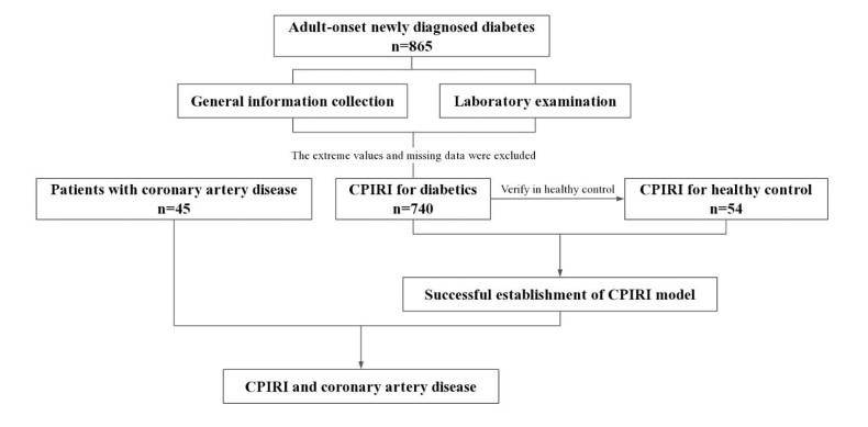
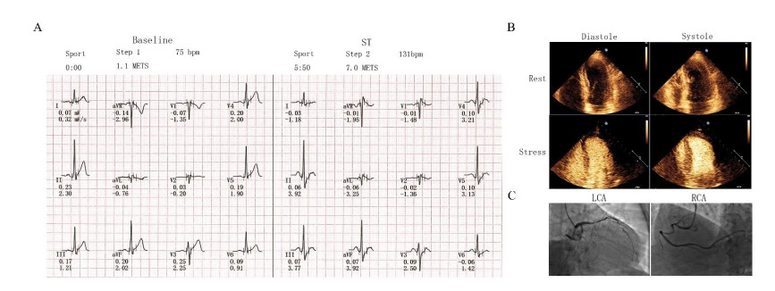
A total of 865 adults diagnosed with new-onset diabetes mellitus (DM) within one year and 54 healthy controls (HC) were recruited to develop a CPIRI model. The CPIRI model was established with fasting C/I as the independent variable and homeostasis model assessment of insulin resistance (HOMA-IR) as the dependent variable. Associations between the CPIRI model and the severity of CAD events were also assessed in 45 hyperglycemic patients with CAD documented via coronary arteriography (CAG) and whom underwent stress echocardiography (SE) and exercise electrocardiography test (EET).
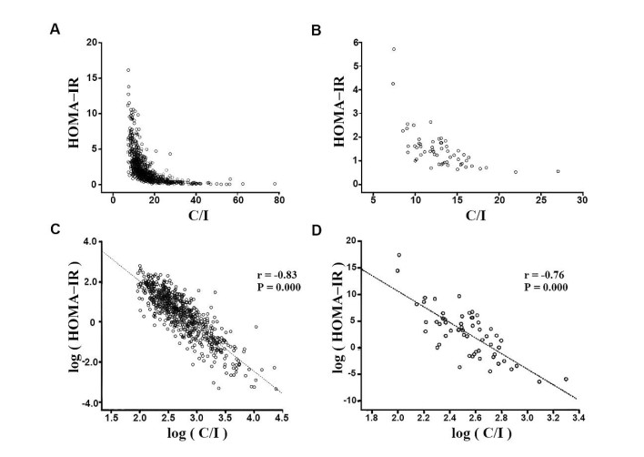
Fasting C-peptide/insulin and HOMA-IR were hyperbolically correlated in DM patients and HC, and log(C/I) and log(HOMA-IR) were linearly and negatively correlated. The respective correlational coefficients were −0.83 (p < 0.001) and −0.76 (p < 0.001). The equations CPIRI(DM) = 670/(C/I)2.24 + 0.25 and CPIRI(HC) = 670/(C/I)2.24 − 1 (F = 1904.39, p < 0.001) were obtained. Patients with insulin resistance exhibited severe coronary artery impairment and myocardial ischemia. In CAD patients there was no significant correlation between insulin resistance and the number of vessels involved.
CPIRI can be used to effectively evaluate insulin resistance, and the combination of CPIRI and non-invasive cardiovascular examination is of great clinical value in the assessment of CAD.
Citation: Hao Dai, Qi Fu, Heng Chen, Mei Zhang, Min Sun, Yong Gu, Ningtian Zhou, Tao Yang. A novel numerical model of combination levels of C-peptide and insulin in coronary artery disease risk prediction[J]. Mathematical Biosciences and Engineering, 2021, 18(3): 2675-2687. doi: 10.3934/mbe.2021136
Insulin resistance is a major risk factor for coronary artery disease (CAD). The C-peptide-to-insulin ratio (C/I) is associated with hepatic insulin clearance and insulin resistance. The current study was designed to establish a novel C/I index (CPIRI) model and provide early risk assessment of CAD.
A total of 865 adults diagnosed with new-onset diabetes mellitus (DM) within one year and 54 healthy controls (HC) were recruited to develop a CPIRI model. The CPIRI model was established with fasting C/I as the independent variable and homeostasis model assessment of insulin resistance (HOMA-IR) as the dependent variable. Associations between the CPIRI model and the severity of CAD events were also assessed in 45 hyperglycemic patients with CAD documented via coronary arteriography (CAG) and whom underwent stress echocardiography (SE) and exercise electrocardiography test (EET).
Fasting C-peptide/insulin and HOMA-IR were hyperbolically correlated in DM patients and HC, and log(C/I) and log(HOMA-IR) were linearly and negatively correlated. The respective correlational coefficients were −0.83 (p < 0.001) and −0.76 (p < 0.001). The equations CPIRI(DM) = 670/(C/I)2.24 + 0.25 and CPIRI(HC) = 670/(C/I)2.24 − 1 (F = 1904.39, p < 0.001) were obtained. Patients with insulin resistance exhibited severe coronary artery impairment and myocardial ischemia. In CAD patients there was no significant correlation between insulin resistance and the number of vessels involved.
CPIRI can be used to effectively evaluate insulin resistance, and the combination of CPIRI and non-invasive cardiovascular examination is of great clinical value in the assessment of CAD.

| [1] |
D. J. Hunter, K. S. Reddy, Noncommunicable diseases, N. Engl. J. Med., 369 (2013), 1336–1343. doi: 10.1056/NEJMra1109345

|
| [2] | Q. Huang, J. H. Wang, D. F. Li, J. H. Zhao, X. J. Feng, N. T. Zhou, Exercise electrocardiography combined with stress echocardiography for predicting myocardial ischemia in adults, Exp. Ther. Med., 21 (2021), 130. |
| [3] | K. E. Bornfeldt, I. Tabas, Insulin resistance, hyperglycemia, and atherosclerosis, Cell Metab., 14 (2011), 575-585. |
| [4] | F. C. Sasso, P. C. Pafundi, R. Marfella, P. Calabrò, F. Piscione, F. Furbatto, et al., Adiponectin and insulin resistance are related to restenosis and overall new PCI in subjects with normal glucose tolerance: the prospective AIRE Study, Cardiovasc. Diabetol., 18 (2019), 24. |
| [5] | K. Esposito, M. Ciotola, F. C. Sasso, D. Cozzolino, F. Saccomanno, R. Assaloni, et al., Effect of a single high-fat meal on endothelial function in patients with the metabolic syndrome: role of tumor necrosis factor-alpha, Nutr. Metab. Cardiovasc. Dis., 17 (2007), 274–279. |
| [6] | H. A. Qazmooz, H. N. Smesam, R. F. Mousa, H. K. Al-Hakeim, M. Maes, Trace element, immune and opioid biomarkers of unstable angina, increased atherogenicity and insulin resistance: Results of machine learning, J. Trace. Elem. Med. Biol., 64 (2021), 126703. |
| [7] | D. Cozzolino, G. Sessa, T. Salvatore, F.C. Sasso, D. Giugliano, P. J. Lefebvre, R. Torella, et al., The involvement of the opioid system in human obesity: a study in normal weight relatives of obese people, J. Clin. Endocrinol. Metab., 81 (1996), 713–718. |
| [8] |
R. Marfella, M. D'. Amico, C. D. Filippo, M. Siniscalchi, F. C. Sasso, F. Ferraraccio, et al., The possible role of the ubiquitin proteasome system in the development of atherosclerosis in diabetes, Cardiovasc. Diabetol., 6 (2007), 35. doi: 10.1186/1475-2840-6-35
|
| [9] | D. Torella, G. M. Ellison, M. Torella, C. Vicinanza, I. Aquila, C. Iaconetti, et al., Carbonic anhydrase activation is associated with worsened pathological remodeling in human ischemic diabetic cardiomyopathy, J. Am. Heart Assoc., 3 (2014), e000434. |
| [10] |
R. Marfella, F. Ferraraccio, M. R. Rizzo, M. Portoghese, M. Barbieri, C. Basilio, et al., Innate immune activity in plaque of patients with untreated and L-thyroxine-treated subclinical hypothyroidism, J. Clin. Endocrinol. Metab., 96 (2011), 1015–1020. doi: 10.1210/jc.2010-1382
|
| [11] |
R. Marfella, F. C. Sasso, M. Siniscalchi, P. Paolisso, M. R. Rizzo, F. Ferraro, et al., Peri-procedural tight glycemic control during early percutaneous coronary intervention is associated with a lower rate of in-stent restenosis in patients with acute ST-elevation myocardial infarction, J. Clin. Endocrinol. Metab., 97 (2012), 2862–2871. doi: 10.1210/jc.2012-1364
|
| [12] |
G. Reaven, Insulin resistance and coronary heart disease in nondiabetic individuals, Arterioscler. Thromb. Vasc. Biol., 32 (2012), 1754–1759. doi: 10.1161/ATVBAHA.111.241885
|
| [13] |
H. P. Himsworth, Diabetes mellitus: its differentiation into insulin-sensitive and insulin-insensitive types, Int. J. Epidemiol., 42 (2013), 1594–1598. doi: 10.1093/ije/dyt203
|
| [14] |
S. E. Kahn, R. L. Hull, K. M. Utzschneider, Mechanisms linking obesity to insulin resistance and type 2 diabetes, Nature, 444 (2006), 840–846. doi: 10.1038/nature05482
|
| [15] |
B. B. Kahn, J. S. Flier, Obesity and insulin resistance, J. Clin. Invest., 106 (2000), 473–481. doi: 10.1172/JCI10842
|
| [16] | C. J. Ramnanan, D. S. Edgerton, G. Kraft, A. D. Cherrington, Physiologic action of glucagon on liver glucose metabolism, Diabetes Obes. Metab., 13 (2011), 118–125. |
| [17] |
H. V. Lin, D. Accili, Hormonal regulation of hepatic glucose production in health and disease, Cell Metab., 14 (2011), 9–19. doi: 10.1016/j.cmet.2011.06.003
|
| [18] |
D. R. Matthews, J. P. Hosker, A. S. Rudenski, B. A. Naylor, D. F. Treacher, R. C. Turner, Homeostasis model assessment: insulin resistance and beta-cell function from fasting plasma glucose and insulin concentrations in man, Diabetologia, 28 (1985), 412–419. doi: 10.1007/BF00280883
|
| [19] |
T. M. Wallace, J. C. Levy, D. R. Matthews, Use and abuse of HOMA modeling, Diabetes Care, 27 (2004), 1487–1495. doi: 10.2337/diacare.27.6.1487
|
| [20] |
J. Wahren, A. Kallas, A. A. Sima, The clinical potential of C-peptide replacement in type 1 diabetes, Diabetes, 61 (2012), 761–772. doi: 10.2337/db11-1423
|
| [21] |
O. K. Faber, H. Kehlet, S. Madsbad, C. Binder, Kinetics of human C-peptide in man, Diabetes, 27 (1978), 207–209. doi: 10.2337/diab.27.1.S207
|
| [22] |
G. L. C. Yosten, C. Maric-Bilkan, P. Luppi, J. Wahren, Physiological effects and therapeutic potential of proinsulin C-peptide, Am. J. Physiol. Endocrinol. Metab., 307 (2014), E955–968. doi: 10.1152/ajpendo.00130.2014
|
| [23] |
R. R. Henry, G. Brechtel, K. Griver, Secretion and hepatic extraction of insulin after weight loss in obese noninsulin-dependent diabetes mellitus, J. Clin. Endocrinol. Metab., 66 (1988), 979–986. doi: 10.1210/jcem-66-5-979
|
| [24] | J. Jimenez, S. Zuniga-Guajardo, B. Zinman, A. Angel, Effects of weight loss in massive obesity on insulin and C-peptide dynamics: sequential changes in insulin production, clearance, and sensitivity, J. Clin. Endocrinol. Metab., 64 (1987), 661–668. |
| [25] | M. T. Meistas, S. Margolis, A. A. Kowarski, Hyperinsulinemia of obesity is due to decreased clearance of insulin, Am. J. Physiol., 245 (1983), E155–159. |
| [26] | A. Katz, S. S. Nambi, K. Mather, A. D. Baron, D. A. Follmann, G. Sullivan, et al., Quantitative insulin sensitivity check index: a simple, accurate method for assessing insulin sensitivity in humans, J. Clin. Endocrinol. Metab., 85 (2000), 2402–2410. |
| [27] |
I. R. Mordi, A. A. Badar, R. J. Irving, J. R. Weir-McCall, J. G. Houston, C. C. Lang, Efficacy of noninvasive cardiac imaging tests in diagnosis and management of stable coronary artery disease, Vasc. Health Risk Manag., 13 (2017), 427–437. doi: 10.2147/VHRM.S106838
|
| [28] |
E. Bonora, S. Kiechl, J. Willeit, F. Oberhollenzer, G. Egger, J. B. Meigs, et al., Insulin resistance as estimated by homeostasis model assessment predicts incident symptomatic cardiovascular disease in caucasian subjects from the general population: the Bruneck study, Diabetes Care, 30 (2007), 318–324. doi: 10.2337/dc06-0919
|
| [29] |
E. Bonora, G. Formentini, F. Calcaterra, S. Lombardi, F. Marini, L. Zenari, et al., HOMA-estimated insulin resistance is an independent predictor of cardiovascular disease in type 2 diabetic subjects: prospective data from the Verona Diabetes Complications Study, Diabetes Care, 25 (2002), 1135–1141. doi: 10.2337/diacare.25.7.1135
|
| [30] |
K. S. Polonsky, A. H. Rubenstein, C-peptide as a measure of the secretion and hepatic extraction of insulin: Pitfalls and limitations, Diabetes, 33 (1984), 486–494. doi: 10.2337/diab.33.5.486
|
| [31] | R. H. Broh-Kahn, I. A. Mirsky, The inactivation of insulin by tissue extracts; the effect of fasting on the insulinase content of rat liver, Arch. Biochem., 20 (1949), 10–14. |
| [32] |
O. Pivovarova, W. Bernigau, T. Bobbert, F. Isken, M. Möhlig, J. Spranger, et al., Hepatic insulin clearance is closely related to metabolic syndrome components, Diabetes Care, 36(2013), 3779–3785. doi: 10.2337/dc12-1203
|
| [33] | C. W. Hilton, H. Mizuma, F. Svec, C. Prasad, Relationship between plasma cyclo (His-Pro), a neuropeptide common to processed protein-rich food, and C-peptide/insulin molar ratio in obese women, Nutr. Neurosci., 4 (2001), 469–474. |
| [34] |
A. M. Lundsgaard, K. A. Sjøberg, L. D. Høeg, J. Jeppesen, A. B. Jordy, A. K. Serup, et al., Opposite Regulation of Insulin Sensitivity by Dietary Lipid Versus Carbohydrate Excess, Diabetes, 66 (2017), 2583–2595. doi: 10.2337/db17-0046
|
| [35] |
T. M. Zilkens, A. M. Eberle, H. Schmidt-Gayk, Immunoluminometric assay (ILMA) for intact human proinsulin and its conversion intermediates, Clin. Chim. Acta., 247 (1996), 23–37. doi: 10.1016/0009-8981(95)06217-3
|
| [36] |
N. Li, P. T. Katzmarzyk, R. Horswell, Y. Zhang, W. Li, W. Zhao, et al., BMI and coronary heart disease risk among low-income and underinsured diabetic patients, Diabetes Care, 37 (2014), 3204–3212. doi: 10.2337/dc14-1091
|
| [37] |
M. C. G. J. Brouwers, N. Simons, C. D. A. Stehouwer, A. Isaacs, Non-alcoholic fatty liver disease and cardiovascular disease: assessing the evidence for causality, Diabetologia, 63 (2020), 253–260. doi: 10.1007/s00125-019-05024-3
|
| [38] |
I. Kowalska, J. Prokop, H. Bachórzewska-Gajewska, B. Telejko, I. Kinalskal, W. Kochman, et al., Disturbances of glucose metabolism in men referred for coronary arteriography: Postload glycemia as predictor for coronary atherosclerosis, Diabetes Care, 24 (2001), 897–901. doi: 10.2337/diacare.24.5.897
|
| [39] |
F. C. Sasso, O. Carbonara, R. Nasti, B. Campana, R. Marfella, M. Torella, et al., Glucose metabolism and coronary heart disease in patients with normal glucose tolerance, Jama, 291 (2004), 1857–1863. doi: 10.1001/jama.291.15.1857
|
| [40] |
T. Strisciuglio, R. Izzo, E. Barbato, G. D. Gioia, I. Colaiori, A. Fiordelisi, et al., Insulin resistance predicts severity of coronary atherosclerotic disease in non-diabetic patients, J. Clin. Med., 9 (2020), 2144. doi: 10.3390/jcm9072144
|
 mbe-18-03-136-Supplementary.pdf mbe-18-03-136-Supplementary.pdf |
 |
Figures(4) / Tables(1)

Hao Dai, Qi Fu, Heng Chen, Mei Zhang, Min Sun, Yong Gu, Ningtian Zhou, Tao Yang. A novel numerical model of combination levels of C-peptide and insulin in coronary artery disease risk prediction[J]. Mathematical Biosciences and Engineering, 2021, 18(3): 2675-2687. doi: 10.3934/mbe.2021136


 DownLoad: