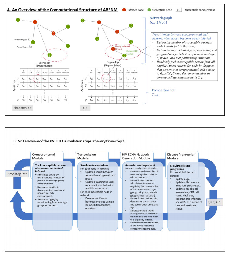
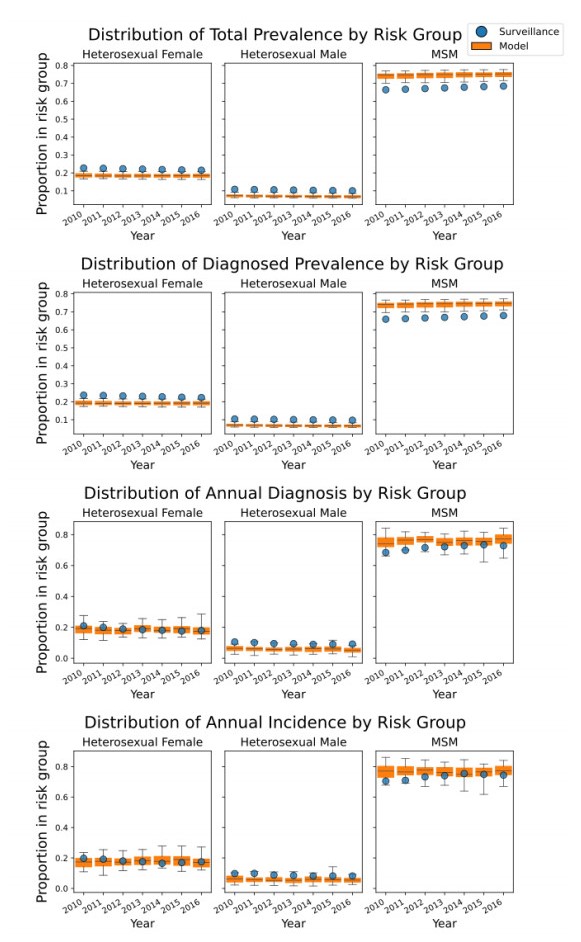
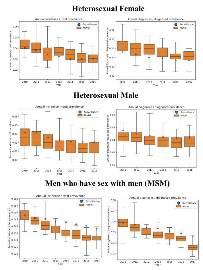
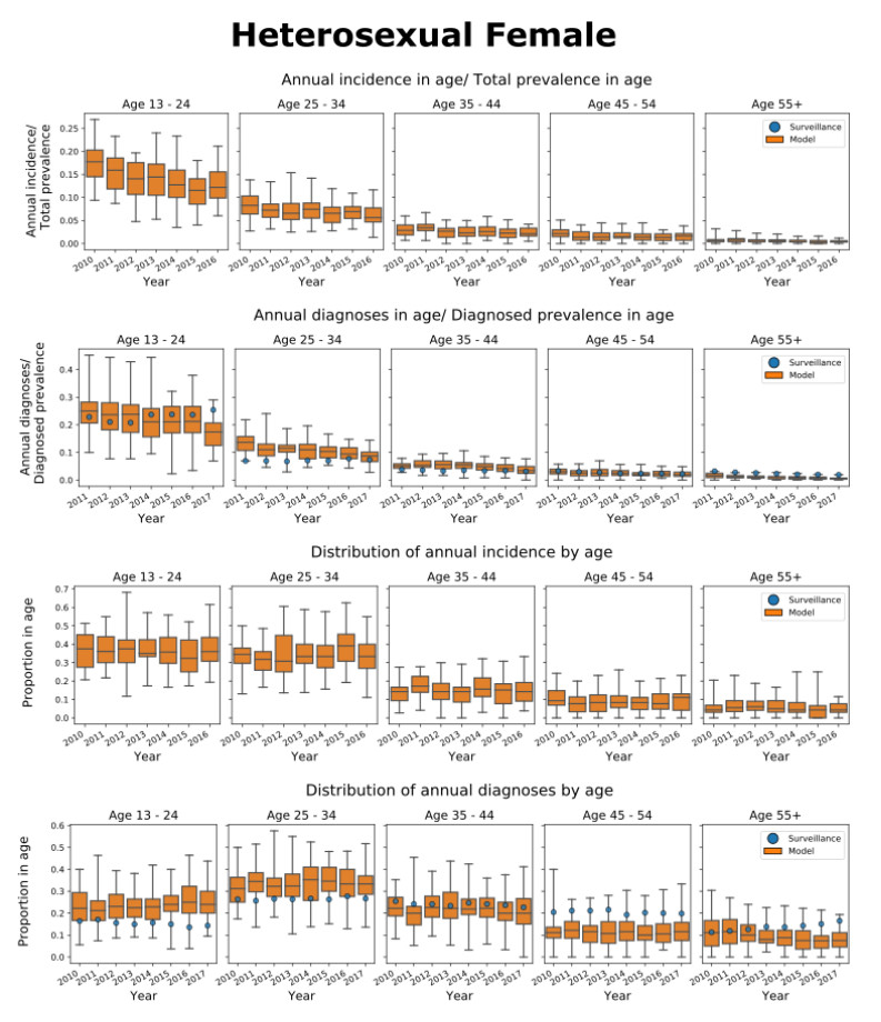
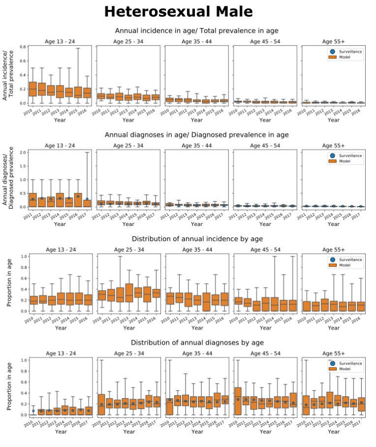
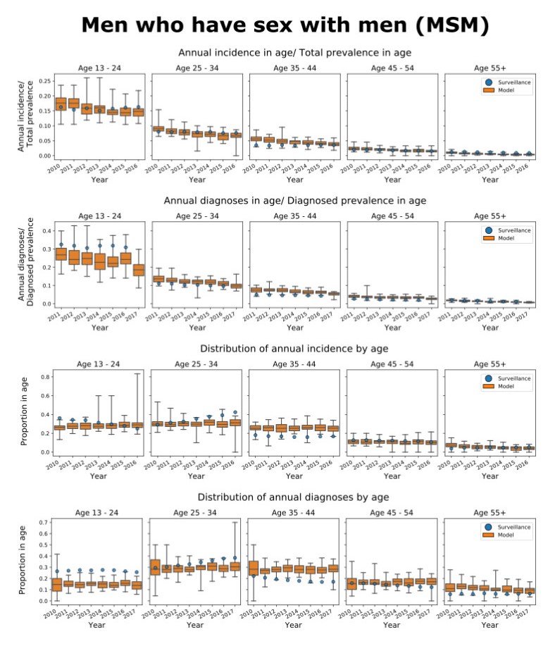
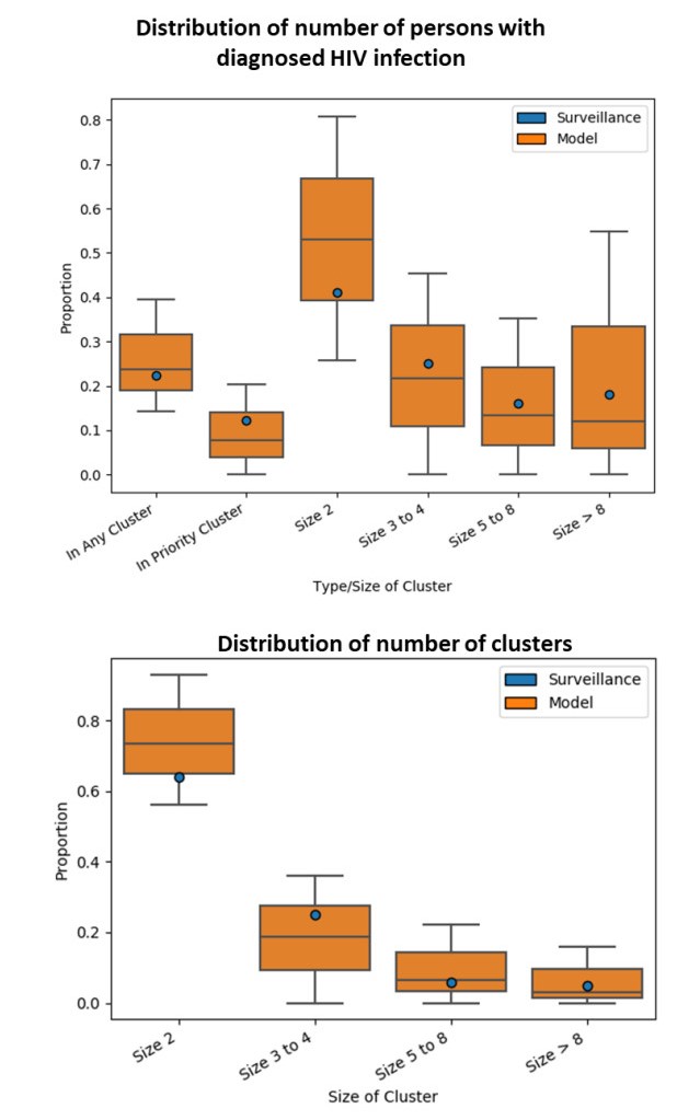
We present the Progression and Transmission of HIV (PATH 4.0), a simulation tool for analyses of cluster detection and intervention strategies. Molecular clusters are groups of HIV infections that are genetically similar, indicating rapid HIV transmission where HIV prevention resources are needed to improve health outcomes and prevent new infections. PATH 4.0 was constructed using a newly developed agent-based evolving network modeling (ABENM) technique and evolving contact network algorithm (ECNA) for generating scale-free networks. ABENM and ECNA were developed to facilitate simulation of transmission networks for low-prevalence diseases, such as HIV, which creates computational challenges for current network simulation techniques. Simulating transmission networks is essential for studying network dynamics, including clusters. We validated PATH 4.0 by comparing simulated projections of HIV diagnoses with estimates from the National HIV Surveillance System (NHSS) for 2010–2017. We also applied a cluster generation algorithm to PATH 4.0 to estimate cluster features, including the distribution of persons with diagnosed HIV infection by cluster status and size and the size distribution of clusters. Simulated features matched well with NHSS estimates, which used molecular methods to detect clusters among HIV nucleotide sequences of persons with HIV diagnosed during 2015–2017. Cluster detection and response is a component of the U.S. Ending the HIV Epidemic strategy. While surveillance is critical for detecting clusters, a model in conjunction with surveillance can allow us to refine cluster detection methods, understand factors associated with cluster growth, and assess interventions to inform effective response strategies. As surveillance data are only available for cases that are diagnosed and reported, a model is a critical tool to understand the true size of clusters and assess key questions, such as the relative contributions of clusters to onward transmissions. We believe PATH 4.0 is the first modeling tool available to assess cluster detection and response at the national-level and could help inform the national strategic plan.
Citation: Sonza Singh, Anne Marie France, Yao-Hsuan Chen, Paul G. Farnham, Alexandra M. Oster, Chaitra Gopalappa. Progression and transmission of HIV (PATH 4.0)-A new agent-based evolving network simulation for modeling HIV transmission clusters[J]. Mathematical Biosciences and Engineering, 2021, 18(3): 2150-2181. doi: 10.3934/mbe.2021109
We present the Progression and Transmission of HIV (PATH 4.0), a simulation tool for analyses of cluster detection and intervention strategies. Molecular clusters are groups of HIV infections that are genetically similar, indicating rapid HIV transmission where HIV prevention resources are needed to improve health outcomes and prevent new infections. PATH 4.0 was constructed using a newly developed agent-based evolving network modeling (ABENM) technique and evolving contact network algorithm (ECNA) for generating scale-free networks. ABENM and ECNA were developed to facilitate simulation of transmission networks for low-prevalence diseases, such as HIV, which creates computational challenges for current network simulation techniques. Simulating transmission networks is essential for studying network dynamics, including clusters. We validated PATH 4.0 by comparing simulated projections of HIV diagnoses with estimates from the National HIV Surveillance System (NHSS) for 2010–2017. We also applied a cluster generation algorithm to PATH 4.0 to estimate cluster features, including the distribution of persons with diagnosed HIV infection by cluster status and size and the size distribution of clusters. Simulated features matched well with NHSS estimates, which used molecular methods to detect clusters among HIV nucleotide sequences of persons with HIV diagnosed during 2015–2017. Cluster detection and response is a component of the U.S. Ending the HIV Epidemic strategy. While surveillance is critical for detecting clusters, a model in conjunction with surveillance can allow us to refine cluster detection methods, understand factors associated with cluster growth, and assess interventions to inform effective response strategies. As surveillance data are only available for cases that are diagnosed and reported, a model is a critical tool to understand the true size of clusters and assess key questions, such as the relative contributions of clusters to onward transmissions. We believe PATH 4.0 is the first modeling tool available to assess cluster detection and response at the national-level and could help inform the national strategic plan.

| [1] | Centers for Disease Control and Prevention. Estimated HIV incidence and prevalence in the United States, 2014-2018. HIV Surveillance Supplemental Report 2020; 25(No. 1). Available from: http://www.cdc.gov/hiv/library/reports/hiv-surveillance.html. Published May 2020. Accessed July 2020. |
| [2] | Centers for Disease Control and Prevention. HIV Surveillance Report, 2018 (Updated); vol.31. Available from: https://www.cdc.gov/hiv/pdf/library/reports/surveillance/cdc-hiv-surveillance-report-2018-updated-vol-31.pdf. Published May 2020. Accessed September 2020. |
| [3] |
P. G. Farnham, D. R. Holtgrave, C. Gopalappa, A. B. Hutchinson, S. L. Sansom, Lifetime costs and quality-adjusted life years saved from HIV prevention in the test and treat era, J. Acquir. Immune Defic. Syndr., 64 (2013), e15-18. doi: 10.1097/QAI.0b013e3182a5c8d4 doi: 10.1097/QAI.0b013e3182a5c8d4

|
| [4] |
N. S. Harris, A. S. Johnson, Y. A. Huang, D. Kern, P. Fulton, D. K. Smith, et al., Vital signs: Status of human immunodeficiency virus testing, viral suppression, and HIV preexposure prophylaxis-United States, 2013-2018. MMWR Morb. Mortal Wkly. Rep., 68 (2019), 1117-1123. doi: 10.15585/mmwr.mm6848e1
|
| [5] | Centers for Disease Control and Prevention. Effectiveness of Prevention Strategies to Reduce the Risk of Acquiring or Transmitting HIV. Available from: https://www.cdc.gov/hiv/risk/estimates/preventionstrategies.html Accessed May 2020. |
| [6] |
C. Gopalappa, P. G. Farnham, Y. H. Chen, S. L. Sansom, Progression and Transmission of HIV/AIDS (PATH 2.0), Med. Decis. Making., 37 (2017), 224-233. doi: 10.1177/0272989X16668509 doi: 10.1177/0272989X16668509
|
| [7] |
N. Khurana, E. Yaylali, P. G. Farnham, K. A. Hicks, B. T. Allaire, E. Jacobson, et al., Impact of improved HIV care and treatment on PrEP effectiveness in the United States, 2016-2020, J. Acquir. Immune Defic. Syndr., 78 (2018), 399-405. doi: 10.1097/QAI.0000000000001707 doi: 10.1097/QAI.0000000000001707
|
| [8] | H. W. Hethcote, J. W. Van Ark, Modeling HIV transmission and AIDS in the United States, Springer Sci. Business Media, 95 (2013). |
| [9] |
Z. Li, D. W. Purcell, S. L. Sansom, D. Hayes, H. I. Hall, Vital signs: HIV transmission along the continuum of care - United States, 2016. MMWR Morb. Mortal Wkly. Rep., 68 (2019), 267-272. doi: 10.15585/mmwr.mm6811e1
|
| [10] |
E. F. Long, M. L. Brandeau, D. K. Owens, The cost-effectiveness and population outcomes of expanded HIV screening and antiretroviral treatment in the United States, Ann. Intern. Med., 153 (2010), 778-789. doi: 10.7326/0003-4819-153-12-201012210-00004 doi: 10.7326/0003-4819-153-12-201012210-00004
|
| [11] |
J. A. Jacquez, C. P. Simon, J. Koopman, L. Sattenspiel, T. Perry, Modeling and analyzing HIV transmission: The effect of contact patterns, Math. Biosci., 92 (1988). doi: 10.1016/0025-5564(88)90031-4 doi: 10.1016/0025-5564(88)90031-4
|
| [12] |
E. A. Hernandez-Vargas, R. H. Middleton, Modeling the three stages in HIV infection, J. Theor. Biol., 320 (2013), 33-40. doi: 10.1016/j.jtbi.2012.11.028 doi: 10.1016/j.jtbi.2012.11.028
|
| [13] |
A. Lasry, S. L. Sansom, K. A. Hicks, V. Uzunangelov, A model for allocating CDC's HIV prevention resources in the United States, Health Care Manag. Sci., 14 (2011), 115-124. doi: 10.1007/s10729-010-9147-2 doi: 10.1007/s10729-010-9147-2
|
| [14] |
S. W. Sorensen, S. L. Sansom, J. T. Brooks, G. Marks, E. M. Begier, K. Buchacz, et al., A mathematical model of comprehensive test-and-treat services and HIV incidence among men who have sex with men in the United States, PloS One, 7 (2012), e29098. doi: 10.1371/journal.pone.0029098 doi: 10.1371/journal.pone.0029098
|
| [15] |
D. R. Holtgrave, Development of year 2020 goals for the National HIV/AIDS Strategy for the United States, AIDS Behav., 18 (2014), 638-643. doi: 10.1007/s10461-013-0579-9 doi: 10.1007/s10461-013-0579-9
|
| [16] |
B. M. Adams, H. T. Banks, M. Davidian, H-D. Kwon, H. T. Tran, S. N. Wynne, et al., HIV dynamics: modeling, data analysis, and optimal treatment protocols, J. Comput. Appl. Math., 184 (2005), 10-49. doi: 10.1016/j.cam.2005.02.004
|
| [17] | E. Uzun Jacobson, K. A. Hicks, E. L. Tucker, P. G. Farnham, S. L. Sansom, Effects of reaching national goals on HIV incidence, by race and ethnicity, in the United States, J. Public Health Manag. Pract., 24 (2018), E1-E8. |
| [18] |
A. M. Oster, A. M. France, J. Mermin, Molecular epidemiology and the transformation of HIV prevention, JAMA, 319 (2018), 1657-1658. doi: 10.1001/jama.2018.1513 doi: 10.1001/jama.2018.1513
|
| [19] |
A. M. Oster, A. M. France, N. Panneer, M. C. Bañez Ocfemia, E. Campbell, S. Dasgupta, et al., Identifying clusters of recent and rapid HIV transmission through analysis of molecular surveillance data, J. Acquir. Immune Defic. Syndr., 79 (2018), 543-550. doi: 10.1097/QAI.0000000000001856 doi: 10.1097/QAI.0000000000001856
|
| [20] |
A. S. Fauci, R. R. Redfield, G. Sigounas, M. D. Weahkee, B. P. Giroir, Ending the HIV epidemic: A plan for the United States, JAMA, 321 (2019), 844-845. doi: 10.1001/jama.2019.1343
|
| [21] |
R. Chou, C. Evans, A. Hoverman, C. Sun, T. Dana, C. Bougatsos, et al., Preexposure prophylaxis for the prevention of HIV infection, JAMA, 321 (2019), 2214-2230. doi: 10.1001/jama.2019.2591 doi: 10.1001/jama.2019.2591
|
| [22] |
J. M. Baeten, D. Donnell, P. Ndase, N. R. Mugo, J. D. Campbell, J. Wangisi, et al., Antiretroviral prophylaxis for HIV prevention in heterosexual men and women, N. Engl. J. Med., 367 (2012), 399-410. doi: 10.1056/NEJMoa1108524 doi: 10.1056/NEJMoa1108524
|
| [23] |
R. M. Grant, J. R. Lama, P. L. Anderson, V. McMahan, A. Y. Liu, L. Vargas, et al., Preexposure chemoprophylaxis for HIV prevention in men who have sex with men, N. Engl. J. Med., 363 (2010), 2587-2599. doi: 10.1056/NEJMoa1011205 doi: 10.1056/NEJMoa1011205
|
| [24] |
M. C. Thigpen, P. M. Kebaabetswe, L. A. Paxton, D. K. Smith, S. R. Pathak, F. A. Soud, et al., Antiretroviral preexposure prophylaxis for heterosexual HIV transmission in Botswana, N. Engl. J. Med., 367 (2012), 423-434. doi: 10.1056/NEJMoa1110711 doi: 10.1056/NEJMoa1110711
|
| [25] |
S. L. Sansom, K. A. Hicks, J. Carrico, E. U. Jacobson, R. K. Shrestha, T. A. Green, et al., Optimal allocation of docietal HIV prevention resources to reduce HIV incidence in the United States, Am. J. Public Health., 111 (2021), 150-158. doi: 10.2105/AJPH.2020.305965 doi: 10.2105/AJPH.2020.305965
|
| [26] |
D. R. Gibson, N. M. Flynn, D. Perales, Effectiveness of syringe exchange programs in reducingHIV risk behavior and HIV seroconversion among injecting drug users, AIDS., 15 (2001), 1329-1341. doi: 10.1097/00002030-200107270-00002 doi: 10.1097/00002030-200107270-00002
|
| [27] |
R. M. Fernandes, M. Cary, G. Duarte, G. Jesus, J. Alarcão, C. Torre, et al., Effectiveness of needle and syringe Programmes in people who inject drugs-An overview of systematic reviews, BMC Public Health, 17 (2017), 309. doi: 10.1186/s12889-017-4210-2 doi: 10.1186/s12889-017-4210-2
|
| [28] |
M. Adams, Q. An, D. Broz, J. Burnett, C. Wejnert, G. Paz-Bailey, NHBS Study Group, Distributive syringe sharing and use of syringe services programs (SSPs) among persons who inject drugs, AIDS Behav., 23 (2019), 3306-3314. doi: 10.1007/s10461-019-02615-4 doi: 10.1007/s10461-019-02615-4
|
| [29] |
E. J. Aspinall, D. Nambiar, D. J. Goldberg, M. Hickman, A. Weir, E. Van Velzen, et al., Are needle and syringe programmes associated with a reduction in HIV transmission among people who inject drugs: A systematic review and meta-analysis, Int. J. Epidemiol., 43 (2014), 235-248. doi: 10.1093/ije/dyt243 doi: 10.1093/ije/dyt243
|
| [30] | D. des Jarlais, A. Nugent, A. Solberg, J. Feelemyer, J. Mermin, D. Holtzman, Syringe service programs for persons who inject drugs in urban, suburban, and rural areas-United States, 2013, MMWR Morb. Mortal Wkly. Rep., 64 (2015), 1337-1341. |
| [31] | M. Eden, R. Castonguay, B. Munkhbat, H. Balasubramanian, C. Gopalappa., Agent-based evolving network modeling: A new simulation method for modeling diseases with low prevalence, Health Care Manag. Sci., (2019). In Press. |
| [32] |
C. I. Siettos, L. Russo, Mathematical modeling of infectious disease dynamics, Virulence, 4 (2013), 295-306. doi: 10.4161/viru.24041 doi: 10.4161/viru.24041
|
| [33] |
T. Smieszek, L. Fiebig, R. W. Scholz, Models of epidemics: When contact repetition and clustering should be included, Theor. Biol. Med. Model., 6 (2009), 11. doi: 10.1186/1742-4682-6-11 doi: 10.1186/1742-4682-6-11
|
| [34] |
A-L. Barabasi, R. Albert, Emergence of scaling in random networks, Science (New York, NY), 286 (1999), 509-512. doi: 10.1126/science.286.5439.509 doi: 10.1126/science.286.5439.509
|
| [35] |
A. M. El-Sayed, P. Scarborough, L. Seemann, S. Galea, Social network analysis and agent-based modeling in social epidemiology, Epidemiol. Perspect. Innov., 9 (2012), 1. doi: 10.1186/1742-5573-9-1 doi: 10.1186/1742-5573-9-1
|
| [36] | Centers for Disease Control and Prevention. Estimated HIV incidence and prevalence in the United States, 2010-2015. HIV Surveillance Supplemental Report 2018; 23(No. 1). Available from: https://www.cdc.gov/hiv/pdf/library/reports/surveillance/cdc-hiv-surveillance-supplemental-report-vol-23-1.pdf Published March 2018. Accessed May 2020. |
| [37] |
A. Lansky, T. Finlayson, C. Johnson, D. Holtzman, C. Wejnert, A. Mitsch, et al., Estimating the number of persons who inject drugs in the united states by meta-analysis to calculate national rates of HIV and hepatitis C virus infections, PloS One, 9 (2014), e97596. doi: 10.1371/journal.pone.0097596 doi: 10.1371/journal.pone.0097596
|
| [38] |
D. W. Purcell, C. H. Johnson, A. Lansky, J. Prejean, R. Stein, P. Denning, et al., Estimating the population size of men who have sex with men in the United States to obtain HIV and syphilis rates, Open AIDS J., 6 (2012), 98-107. doi: 10.2174/1874613601206010098 doi: 10.2174/1874613601206010098
|
| [39] |
F. Liljeros, C. R. Edling, L. A. Amaral, H. E. Stanley, Y. Åberg, The web of human sexual contacts, Nature, 411 (2001), 907-908. doi: 10.1038/35082140 doi: 10.1038/35082140
|
| [40] |
J. O. Wertheim, S. L. Kosakovsky Pond, L. A. Forgione, S. R. Mehta, B. Murrell, S. Shah, et al., Social and genetic networks of HIV-1 transmission in New York City, PloS Pathog., 13 (2017), e1006000. doi: 10.1371/journal.ppat.1006000 doi: 10.1371/journal.ppat.1006000
|
| [41] |
J. O Wertheim, A. J. Leigh Brown, N. L. Hepler, S. R. Mehta, D. D. Richman, D.M. Smith, et al., The global transmission network of HIV-1, J. Infect. Dis., 209 (2014), 304-313. doi: 10.1093/infdis/jit524 doi: 10.1093/infdis/jit524
|
| [42] | B. Fotouhi, M. G. Rabbat, Degree correlation in scale-free graphs, Eur. Phys. J. B., 85 (2013), 510. |
| [43] | Y. H. Chen, A. M. France, P. G. Farnham, S. L. Sansom, C. Gopalappa, A. Oster., Replicating HIV Transmission Clusters in a U.S. HIV Agent-Based Model[abstract]. In: Abstracts: SMDM 40th Annual Meeting; 2018 Oct; Montréal, Québec, Canada. |
| [44] | U. Wilensky, NetLogo.[Internet]. 1999. Available from: http://ccl.northwestern.edu/netlogo/. |
| [45] | A. R. Board, L. Linley, A. M. Oster, M. Watson, R. Song, T. Zhang, et al., Geographic distribution of HIV transmission networks in the United States, J. Acquir. Immune Defic. Syndr., (2020). In Press. |
| [46] | K. Buchacz, C. Armon, F. J. Palella, R. K. Baker, E. Tedaldi, M. D. Durham, et al., CD4 cell counts at HIV diagnosis among HIV outpatient study participants, 2000-2009, AIDS Res. Treat., 2012 (2012), 869841. |
| [47] | T. J. Finlayson, B. Le, A. Smith, K. Bowles, M. Cribbin, I. Miles, et al., Centers for disease control and prevention (CDC), HIV risk, prevention, and testing behaviors among men who have sex with men-National HIV Behavioral Surveillance System, 21 U.S. cities, United States, 2008, MMWR Surveill. Summ., 60 (2011), 1-34. |
| [48] | A. Chandra, W. D. Mosher, C. Copen, C. Sionean, Sexual behavior, sexual attraction, and sexual identity in the United States: Data from the 2006-2008 National Survey of Family Growth, Natl. Health Stat. Report., 36 (2011), 1-36. |
| [49] |
J. A. Grey, K. T. Bernstein, P. S. Sullivan, D. W. Purcell, H. W. Chesson, T. L. Gift, et al., Estimating the population sizes of men who have sex with men in US states and counties using data from the American Community Survey, JMIR Public Health Surveill., 2 (2016), e14. doi: 10.2196/publichealth.5365
|
| [50] |
M. Reece, D. Herbenick, V. Schick, S. A. Sanders, B. Dodge, J. D. Fortenberry, Background and considerations on the national survey of sexual health and behavior (NSSHB) from the investigators, J. Sex. Med., 7 (2010), 243-245. doi: 10.1111/j.1743-6109.2010.02038.x doi: 10.1111/j.1743-6109.2010.02038.x
|
| [51] |
S. M. Cohen, K. M. Gray, M. C. Ocfemia, A. S. Johnson, H. I. Hall, The status of the national HIV surveillance system, United States, 2013, Public Health Rep., 129 (2014), 335-341. doi: 10.1177/003335491412900408 doi: 10.1177/003335491412900408
|
| [52] | Centers for Disease Control and Prevention. Behavioral and Clinical Characteristics of Persons with Diagnosed HIV Infection-Medical Monitoring Project, United States, 2016 Cycle (June 2016-May 2017). HIV Surveillance Special Report 21. Revised edition. Available from: https://www.cdc.gov/hiv/library/reports/hiv-surveillance.html. Published June 2019. Accessed Feb 2021. |
| [53] | Centers for Disease Control and Prevention. Monitoring selected national HIV prevention and care objectives by using HIV surveillance data-United States and 6 dependent areas-2011. HIV Surveillance Supplemental Report 2013; 18(No. 5). Available from: https://www.cdc.gov/hiv/pdf/library/reports/surveillance/cdc-hiv-surveillance-supplemental-report-vol-18-5.pdf Published October 2013. Accessed May 2020. |
| [54] | Centers for Disease Control and Prevention. Monitoring selected national HIV prevention and care objectives by using HIV surveillance data-United States and 6 dependent areas-2012. HIV Surveillance Supplemental Report 2014; 19(No. 3). Available from: https://www.cdc.gov/hiv/pdf/library/reports/surveillance/cdc-hiv-surveillance-supplemental-report-vol-19-3.pdf Published November 2014. Accessed May 2020. |
| [55] | Centers for Disease Control and Prevention. Monitoring selected national HIV prevention and care objectives by using HIV surveillance data-United States and 6 dependent areas, 2015. HIV Surveillance Supplemental Report 2017; 22(No. 2). Available from: https://www.cdc.gov/hiv/pdf/library/reports/surveillance/cdc-hiv-surveillance-supplemental-report-vol-22-2.pdf Published July 2017. Accessed May 2020. |
| [56] | Centers for Disease Control and Prevention. Monitoring selected national HIV prevention and care objectives by using HIV surveillance data-United States and 6 dependent areas, 2014. HIV Surveillance Supplemental Report 2016; 21(No. 4). Available from: https://www.cdc.gov/hiv/pdf/library/reports/surveillance/cdc-hiv-surveillance-supplemental-report-vol-21-4.pdf Published July 2016. Accessed May 2020. |
| [57] | Centers for Disease Control and Prevention. Monitoring selected national HIV prevention and care objectives by using HIV surveillance data-United States and 6 dependent areas-2013. HIV Surveillance Supplemental Report 2015; 20(No. 2). Available from: https://www.cdc.gov/hiv/pdf/library/reports/surveillance/cdc-hiv-surveillance-supplemental-report-vol-20-2.pdf Published July 2015. Accessed May 2020. |
| [58] | Centers for Disease Control and Prevention. Monitoring selected national HIV prevention and care objectives by using HIV surveillance data-United States and 6 dependent areas, 2016. HIV Surveillance Supplemental Report 2018; 23(No. 4). Available from: https://www.cdc.gov/hiv/pdf/library/reports/surveillance/cdc-hiv-surveillance-supplemental-report-vol-23-4.pdf Published June 2018. Accessed May 2020. |
| [59] | Centers for Disease Control and Prevention. Monitoring selected national HIV prevention and care objectives by using HIV surveillance data-United States and 6 dependent areas, 2018. HIV Surveillance Supplemental Report 2020; 25(No. 2). Available from: http://www.cdc.gov/hiv/library/reports/hiv-surveillance.html. Published May 2020. Accessed July 2020. |
| [60] | Centers for Disease Control and Prevention. Monitoring selected national HIV prevention and care objectives by using HIV surveillance data-United States and 6 dependent areas, 2017. HIV Surveillance Supplemental Report 2019; 24(No. 3). Available from: http://www.cdc.gov/hiv/library/reports/hiv-surveillance.html. Published June 2019. Accessed July 2020. |
| [61] |
S. L. K. Pond, S. Weaver, A. J. L. Brown, J. O. Wertheim, HIV-TRACE (TRAnsmission Cluster Engine): A tool for large scale molecular epidemiology of HIV-1 and other rapidly evolving pathogens, Mol. Biol. Evol., 35 (2018), 1812-1819. doi: 10.1093/molbev/msy016 doi: 10.1093/molbev/msy016
|
| [62] | Centers for Disease Control and Prevention. HIV Surveillance Report, 2017; vol. 29. Available from: https://www.cdc.gov/hiv/pdf/library/reports/surveillance/cdc-hiv-surveillance-report-2017-vol-29.pdf. Published November 2018. Accessed September 2020. |
| [63] | Centers for Disease Control and Prevention. NCHHSTP AtlasPlus. Updated 2019. Available from: https://gis.cdc.gov/grasp/nchhstpatlas/tables.html. Accessed July 2020. |
 mbe-18-03-109-appendix.docx mbe-18-03-109-appendix.docx |
 |
Figures(7) / Tables(1)

Sonza Singh, Anne Marie France, Yao-Hsuan Chen, Paul G. Farnham, Alexandra M. Oster, Chaitra Gopalappa. Progression and transmission of HIV (PATH 4.0)-A new agent-based evolving network simulation for modeling HIV transmission clusters[J]. Mathematical Biosciences and Engineering, 2021, 18(3): 2150-2181. doi: 10.3934/mbe.2021109


 DownLoad: