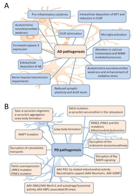
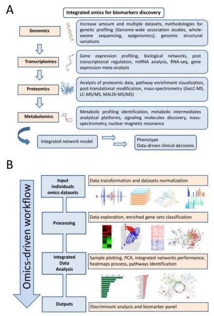
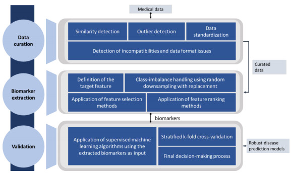
The complexity of biological systems suggests that current definitions of molecular dysfunctions are essential distinctions of a complex phenotype. This is well seen in neurodegenerative diseases (ND), such as Alzheimer's disease (AD) and Parkinson's disease (PD), multi-factorial pathologies characterized by high heterogeneity. These challenges make it necessary to understand the effectiveness of candidate biomarkers for early diagnosis, as well as to obtain a comprehensive mapping of how selective treatment alters the progression of the disorder. A large number of computational methods have been developed to explain network-based approaches by integrating individual components for modeling a complex system. In this review, high-throughput omics methodologies are presented for the identification of potent biomarkers associated with AD and PD pathogenesis as well as for monitoring the response of dysfunctional molecular pathways incorporating multilevel clinical information. In addition, principles for efficient data analysis pipelines are being discussed that can help address current limitations during the experimental process by increasing the reproducibility of benchmarking studies.
Citation: Marios G. Krokidis, Themis P. Exarchos, Panagiotis Vlamos. Data-driven biomarker analysis using computational omics approaches to assess neurodegenerative disease progression[J]. Mathematical Biosciences and Engineering, 2021, 18(2): 1813-1832. doi: 10.3934/mbe.2021094
The complexity of biological systems suggests that current definitions of molecular dysfunctions are essential distinctions of a complex phenotype. This is well seen in neurodegenerative diseases (ND), such as Alzheimer's disease (AD) and Parkinson's disease (PD), multi-factorial pathologies characterized by high heterogeneity. These challenges make it necessary to understand the effectiveness of candidate biomarkers for early diagnosis, as well as to obtain a comprehensive mapping of how selective treatment alters the progression of the disorder. A large number of computational methods have been developed to explain network-based approaches by integrating individual components for modeling a complex system. In this review, high-throughput omics methodologies are presented for the identification of potent biomarkers associated with AD and PD pathogenesis as well as for monitoring the response of dysfunctional molecular pathways incorporating multilevel clinical information. In addition, principles for efficient data analysis pipelines are being discussed that can help address current limitations during the experimental process by increasing the reproducibility of benchmarking studies.

| [1] | C. A. Lane, J. Hardy, J. M Schott, Alzheimer's disease, Eur. J. Neurol., 25 (2017), 59-70. |
| [2] | H. S. Kwon, S. H. Koh, Neuroinflammation in neurodegenerative disorders: the roles of microglia and astrocytes, Transl. Neurodegener., 9 (2020), 42. |
| [3] | C. Marogianni, M. Sokratous, E. Dardiotis, G. M. Hadjigeorgiou, D. Bogdanos, G. Xiromerisiou, Neurodegeneration and inflammation—an interesting interplay in Parkinson's disease, Int. J. Mol. Sci., 21 (2020), 8421. |
| [4] |
S. H. Kim, M. Y. Noh, H. J. Kim, K. W. Oh, J. Park, S. Lee, et al., A therapeutic strategy for Alzheimer's disease focused on immune-inflammatory modulation, Dement Neurocogn. Disord., 18 (2019), 33-46. doi: 10.12779/dnd.2019.18.2.33

|
| [5] | Z. Han, R. Tian, P. Ren, W. Zhou, P. Wang, M. Luo, et al., Parkinson's disease and Alzheimer's disease: a Mendelian randomization study, BMC Med. Genet., 19 (2018), 215. |
| [6] | A. Xie, J. Gao, L. Xu, D. Meng, Shared mechanisms of neurodegeneration in Alzheimer's disease and Parkinson's disease, Biomed. Res. Int., 2014 (2014), 648740. |
| [7] | J. Montaner, L. Ramiro, A. Simats, S. Tiedt, K. Makris, G. C. Jickling, et al., Multilevel omics for the discovery of biomarkers and therapeutic targets for stroke, Nat. Rev. Neurol., 16 (2020), 247-264. |
| [8] | W. J. Lukiw, A. Vergallo, S. Lista, H. Hampel, Y. Zhao, Biomarkers for Alzheimer's disease (AD) and the application of precision medicine, J. Pers. Med., 10 (2020), 138. |
| [9] |
E. M. Cilento, L. Jin, T. Stewart, M. Shi, L. Sheng, J. Zhang, Mass spectrometry: A platform for biomarker discovery and validation for Alzheimer's and Parkinson's diseases, J. Neurochem., 151 (2019), 397-416. doi: 10.1111/jnc.14635
|
| [10] |
J. Verheijen, K. Sleegers, Understanding Alzheimer disease at the interface between genetics and transcriptomics, Trends Genet., 34 (2018), 434-447. doi: 10.1016/j.tig.2018.02.007
|
| [11] |
E. Cuyvers, K. Sleegers, Genetic variations underlying Alzheimer's disease: evidence from genome-wide association studies and beyond, Lancet Neurol., 15 (2016), 857-868. doi: 10.1016/S1474-4422(16)00127-7
|
| [12] | F. L. Heppner, R. M. Ransohoff, B. Becher, Immune attack: The role of inflammation in Alzheimer disease, Nature, 16 (2015), 358-372. |
| [13] | Y. Yan, A. Zhao, Y. Qui, Y. Li, R. Yan, Y. Wang, et al., Genetic association of FERMT2, HLA-DRB1, CD2AP, and PTK2B polymorphisms with Alzheimer's disease risk in the southern Chinese population, Front. Aging Neurosci., 12 (2020), 16. |
| [14] | V. Escott-Price, C. Bellenguez, L. S. Wang, S. H. Choi, D. Harold, L. Jones, et al., Gene-wide analysis detects two new susceptibility genes for Alzheimer's disease. PLoS One, 9 (2014), e94661. |
| [15] | I. López González, P. Garcia-Esparcia, F. Llorens, I. Ferrer, Genetic and transcriptomic profiles of inflammation in neurodegenerative diseases: Alzheimer, Parkinson, Creutzfeldt-Jakob and Tauopathies, Int. J. Mol. Sci., 17 (2016), 206. |
| [16] | Z. P. Van Acker, M. Bretou, Wim Annaert, Endo-lysosomal dysregulations and late-onset Alzheimer's disease: impact of genetic risk factors, Mol. Neurodegener., 14 (2019), 20. |
| [17] | A. De Roeck, C. Van Broeckhoven, K. Sleegers, The role of ABCA7 in Alzheimer's disease: evidence from genomics, transcriptomics and methylomics, Acta Neuropathol., 138 (2019), 201-220. |
| [18] |
C. Reitz, Novel susceptibility loci for Alzheimer's disease, Future Neurol., 10 (2015), 547-558. doi: 10.2217/fnl.15.42
|
| [19] | C. Bellenguez, C. Charbonnier, B. Grenier-Boley, O. Quenez, K. Le Guennec, G. Nicolas, et al., Contribution to Alzheimer's disease risk of rare variants in TREM2, SORL1, and ABCA7 in 1779 cases and 1273 controls, Neurobiol. Aging, 59 (2017), 220.e1-220.e9. |
| [20] |
P. Ciryam, R. Kundra, R. Freer, R. I. Morimoto, C. M. Dobson, M. Vendruscolo, A transcriptional signature of Alzheimer's disease is associated with a metastable subproteome at risk for aggregation, Proc. Natl. Acad. Sci. USA, 113 (2016), 4753-4758. doi: 10.1073/pnas.1516604113
|
| [21] | L. V. Kalia, A. E. Lang, Parkinson's disease, Lancet, 386 (2015), 896-912. |
| [22] | A. Masato, N. Plotegher, D. Boassa, L. Bubacco, Impaired dopamine metabolism in Parkinson's disease pathogenesis, Mol. Neurodegener., 14 (2019), 35. |
| [23] |
M. G. Krokidis, Identification of biomarkers associated with Parkinson's disease by gene expression profiling studies and bioinformatics analysis, AIMS Neurosci., 6 (2019), 333-345. doi: 10.3934/Neuroscience.2019.4.333
|
| [24] | A. Grünewald, K. R. Kumar, C. M. Sue, New insights into the complex role of mitochondria in Parkinson's disease, Prog. Neurobiol., 177 (2019), 79-93. |
| [25] | C. A. D. Costa, W. E. Manaa, E. Duplan, F. Checler, The endoplasmic reticulum stress/unfolded protein response and their contributions to Parkinson's disease physiopathology, Cells, 9 (2020), 2495. |
| [26] | M. Deffains, M. H. Canron, M. Teil, Q. Li, B. Dehay, E. Bezard, et al., L-DOPA regulates α-synuclein accumulation in experimental parkinsonism, Neuropathol. Appl. Neurobiol., 2020. |
| [27] |
L. P. Dolgacheva, A. V. Berezhnov, E. I. Fedotova, V. P. Zinchenko, A. Y. Abramov, Role of DJ-1 in the mechanism of pathogenesis of Parkinson's disease, J. Bioenerg. Biomembr., 51 (2019), 175-188. doi: 10.1007/s10863-019-09798-4
|
| [28] | A. Urbizu, K. Beyer, Epigenetics in Lewy body diseases: Impact on gene expression, utility as a biomarker, and possibilities for therapy, Int. J. Mol. Sci., 21 (2020), 4718. |
| [29] | D. M. O'Hara, G. Pawar, S. K. Kalia, L. V. Kalia, LRRK2 and α-Synuclein: Distinct or synergistic players in Parkinson's disease?, Front. Neurosci., 14 (2020), 577. |
| [30] | T. K. Lin, K. J. Lin, K. L. Lin, C. W. Liou, S. D. Chen, Y. C. Chuang, et al., When friendship turns sour: effective communication between mitochondria and intracellular organelles in Parkinson's disease, Front. Cell. Dev. Biol., 8 (2020), 607392. |
| [31] | B. Wang, K. R. Stanford, M. Kundu, ER-to-Golgi trafficking and its implication in neurological diseases, Cells, 9 (2020), 408. |
| [32] | T. M. Axelsen, D. P. D. Woldbye, Gene therapy for Parkinson's disease, an update, J. Parkinsons Dis., 8 (2018), 195-215. |
| [33] | T. J. Collier, D. E. Jr. Redmond, K. Steece-Collier, J. W. Lipton, F. P. Manfredsson, Is a-synuclein loss-of-function a contributor to parkinsonian pathology? Evidence from non-human primates, Front. Neurosci., 10 (2016), 12. |
| [34] | C. Klein, N. Hattori, C. Marras, MDSGene: Closing data gaps in genotype-phenotype correlations of monogenic Parkinson's disease, J. Parkinsons Dis., 8 (2018), S25-S30. |
| [35] | J. Chi, Q. Xie, J. Jia, X. Liu, J. Sun, Y. Deng, L. Yi, Integrated analysis and identification of novel biomarkers in Parkinson's disease, Front. Aging Neurosci., 10 (2018), 178. |
| [36] | Y. I. Li, G. Wong, J. Humphrey, T. Raj, Prioritizing Parkinson's disease genes using population-scale transcriptomic data, Nat. Commun., 10 (2019), 994. |
| [37] |
K. J. Karczewski, M. P. Snyder, Integrative omics for health and disease, Nat. Rev. Genet., 19 (2018), 299-310. doi: 10.1038/nrg.2018.4
|
| [38] | B. Wang, V. Kumar, A. Olson, D. Ware, Reviving the transcriptome studies: an insight into the emergence of single-molecule transcriptome sequencing, Front. Genet., 10 (2019), 384. |
| [39] | F. R. Pinu, S. A. Goldansaz, J. Jaine, Translational metabolomics: current challenges and future opportunities, Metabolites, 9 (2019), 108. |
| [40] | J. L. Ren, A. H. Zhang, L. Kong, X. J. Wang, Advances in mass spectrometry-based metabolomics for investigation of metabolites, RSC Adv., 8 (2018), 22335. |
| [41] | J. M. Wilkins, E. Trushina, Application of metabolomics in Alzheimer's disease, Front. Neurol., 8 (2018), 719. |
| [42] | E. Trushina, T. Dutta, X. M. Persson, M. M. Mielke, R. C. Petersen, Identification of altered metabolic pathways in plasma and CSF in mild cognitive impairment and Alzheimer's disease using metabolomics, PLoS One, 8 (2013), e63644. |
| [43] |
G. Paglia, M. Stocchero, S. Cacciatore, S. Lai, P. Angel, M. T. Alam, et al., Unbiased metabolomic investigation of Alzheimer's disease brain points to dysregulation of mitochondrial aspartate metabolism, J. Proteome Res., 15 (2016), 608-618. doi: 10.1021/acs.jproteome.5b01020
|
| [44] | S. G. Snowden, A. A. Ebshiana, A. Hye, Y. An, O. Pletnikova, R. O'Brien, et al., Association between fatty acid metabolism in the brain and Alzheimer disease neuropathology and cognitive performance: a nontargeted metabolomic study, PLoS Med., 14 (2017), e1002266. |
| [45] |
S. P. Guiraud, I. Montoliu, L. Da Silva, L. Dayon, A. N. Galindo, J. Corthesy, et al., High-throughput and simultaneous quantitative analysis of homo-cysteine-methionine cycle metabolites and co-factors in blood plasma and cerebrospinal fluid by isotope dilution LC-MS/MS, Anal. Bioanal. Chem., 409 (2017), 295-305. doi: 10.1007/s00216-016-0003-1
|
| [46] |
J. B. Toledo, M. Arnold, G. Kastenmuller, R. Chang, R. A. Baillie, X. Han, et al., Metabolic network failures in Alzheimer's disease-a biochemical road map, Alzheimers Dement., 13 (2017), 965-84. doi: 10.1016/j.jalz.2017.01.020
|
| [47] | S. F. Graham, O. P. Chevallier, C. T. Elliott, C. Holscher, J. Johnston, B. McGuinness, et al., Untargeted metabolomic analysis of human plasma indicates differentially affected polyamine and l-arginine metabolism in mild cognitive impairment subjects converting to Alzheimer's disease, PLoS One, 10 (2015), e0119452. |
| [48] |
M. Mapstone, F. Lin, M. A. Nalls, A. K. Cheema, A. B. Singleton, M. S. Fiandaca, et al., What success can teach us about failure: the plasma metabolome of older adults with superior memory and lessons for Alzheimer's disease, Neurobiol. Aging, 51 (2017), 148-55. doi: 10.1016/j.neurobiolaging.2016.11.007
|
| [49] |
M. Benson, Clinical implications of omics and systems medicine: focus on predictive and individualized treatment, J. Intern. Med., 279 (2016), 229-240. doi: 10.1111/joim.12412
|
| [50] |
C. Evans, J. Hardin, D. M. Stoebel, Selecting between-sample RNA-Seq normalization methods from the perspective of their assumptions, Brief Bioinform., 19 (2018), 776-792. doi: 10.1093/bib/bbx008
|
| [51] | F. Maleki, K. Ovens, D. J. Hogan, A. J. Kusalik, Gene set analysis: challenges, opportunities, and future research, Front. Genet., 11 (2020), 654. |
| [52] | I. Ihnatova, V. Popovici, E. Budinska, A critical comparison of topology-based pathway analysis methods, PLoS One, 13 (2018), e0191154. |
| [53] | N. Xie, L. Zhang, W. Gao, C. Huang, P. E. Huber, X. Zhou, et al., Subpathway-GM: identification of metabolic subpathways via joint power of interesting genes and metabolites and their topologies within pathways, Signal. Transduct. Target. Ther., 5 (2020), 227. |
| [54] |
Q. Yang, S. Wang, E. Dai, S. Zhou, D. Liu, H. Liu, et al., Pathway enrichment analysis approach based on topological structure and updated annotation of pathway, Brief Bioinform., 20 (2019), 168-177. doi: 10.1093/bib/bbx091
|
| [55] |
P. Kong, P. Lei, S. Zhang, D. Li, J. Zhao, B. Zhang, Integrated microarray analysis provided a new insight of the pathogenesis of Parkinson's disease, Neurosci. Lett., 662 (2018), 51-58. doi: 10.1016/j.neulet.2017.09.051
|
| [56] | M. G. Krokidis, P. Vlamos, Transcriptomics in amyotrophic lateral sclerosis, Front. Biosci. (Elite Ed), 10 (2018), 103-121. |
| [57] | L. Bravo-Merodio, L. A. Williams, G. V. Gkoutos, A. Acharjee, Omics biomarker identification pipeline for translational medicine. J. Transl. Med., 17 (2019), 155. |
| [58] |
M. A. Myszczynska, P. N. Ojamies, A. M. B. Lacoste, D. Neil, A. Saffari, R. Mead, et al., Applications of machine learning to diagnosis and treatment of neurodegenerative diseases, Nat. Rev. Neurol., 16 (2020), 440-456. doi: 10.1038/s41582-020-0377-8
|
| [59] | J. Xin, X. Ren, L. Chen, Y. Wang, Identifying network biomarkers based on protein-protein interactions and expression data, BMC Med. Genomics, 8 (2015), S11. |
| [60] |
L. Fu, K. Fu, Analysis of Parkinson's disease pathophysiology using an integrated genomics-bioinformatics approach, Pathophysiology, 22 (2015), 15-29. doi: 10.1016/j.pathophys.2014.10.002
|
| [61] | R. Al-Ouran, Y. W. Wan, C. G. Mangleburg, T. V. Lee, K. Allison, J. M. Shulman, et al., A portal to visualize transcriptome profiles in mouse models of neurological disorders, Genes (Basel), 10 (2019), E759. |
| [62] | J. Kelly, R. Moyeed, C. Carroll, D. Albani, X. Li, Gene expression meta-analysis of Parkinson's disease and its relationship with Alzheimer's disease, Mol. Brain., 12 (2019), 16. |
| [63] | E. Mariani, F. Frabetti, A. Tarozzi, M. C. Pelleri, F. Pizzetti, R. Casadei, Meta-analysis of Parkinson's disease transcriptome data using TRAM software: whole substantia nigra tissue and single dopamine neuron differential gene expression, PLoS One, 11 (2016), e0161567. |
| [64] |
P. Kong, P. Lei, S. Zhang, D. Li, J. Zhao, B. Zhang, Integrated microarray analysis provided a new insight of the pathogenesis of Parkinson's disease, Neurosci. Lett., 662 (2018), 51-58. doi: 10.1016/j.neulet.2017.09.051
|
| [65] |
E. Glaab, Computational systems biology approaches for Parkinson's disease, Cell Tissue Res., 373 (2018), 91-109. doi: 10.1007/s00441-017-2734-5
|
| [66] | T. M. Nguyen, A. Shafi, T. Nguyen, S. Draghici, Identifying significantly impacted pathways: a comprehensive review and assessment, Genome Biol., 20 (2019), 203. |
| [67] | J. Ma, A. Shojaie, G. Michailidis, A comparative study of topology-based pathway enrichment analysis methods, BMC Bioinform., 20 (2019), 546. |
| [68] | C. Gao, H. Sun, T. Wang, M. Tang, N. I. Bohnen, M. L. T. M. Müller, et al., Model-based and model-free machine learning techniques for diagnostic prediction and classification of clinical outcomes in Parkinson's disease, Sci. Rep., 8 (2018), 7129. |
| [69] |
Y. Hu, Z. Pan, Y. Hu, L. Zhang, J. Wang, Network and pathway-based analyses of genes associated with Parkinson's disease, Mol. Neurobiol., 54 (2017), 4452-4465. doi: 10.1007/s12035-016-9998-8
|
Figures(3) / Tables(1)

Marios G. Krokidis, Themis P. Exarchos, Panagiotis Vlamos. Data-driven biomarker analysis using computational omics approaches to assess neurodegenerative disease progression[J]. Mathematical Biosciences and Engineering, 2021, 18(2): 1813-1832. doi: 10.3934/mbe.2021094


 DownLoad: