Notation | Value | |
Λh | 0.0002/day | |
c | 0.0002/day | |
β1 | 0.000044 /day | |
α1 | 0.003 /day | |
μh | 0.00020 /day | |
b | 0.4/day | |
δh | 0.002 /day | |
γ | 0.1/day | |
Λv | 0.08/day | |
β2 | 0.007 /day | |
α2 | 0.02/day | |
μv | 0.2/day | |
bo | 0.01/day |
Citation: Carmen Lok Tung Ho, Peter Oligbu, Olakunle Ojubolamo, Muhammad Pervaiz, Godwin Oligbu. Clinical Characteristics of Children with COVID-19[J]. AIMS Public Health, 2020, 7(2): 258-273. doi: 10.3934/publichealth.2020022
[1] | Jiajia Zhang, Yuanhua Qiao, Yan Zhang . Stability analysis and optimal control of COVID-19 with quarantine and media awareness. Mathematical Biosciences and Engineering, 2022, 19(5): 4911-4932. doi: 10.3934/mbe.2022230 |
[2] | Yan-Xia Dang, Zhi-Peng Qiu, Xue-Zhi Li, Maia Martcheva . Global dynamics of a vector-host epidemic model with age of infection. Mathematical Biosciences and Engineering, 2017, 14(5&6): 1159-1186. doi: 10.3934/mbe.2017060 |
[3] | Xia Wang, Yuming Chen . An age-structured vector-borne disease model with horizontal transmission in the host. Mathematical Biosciences and Engineering, 2018, 15(5): 1099-1116. doi: 10.3934/mbe.2018049 |
[4] | Ling Xue, Caterina Scoglio . Network-level reproduction number and extinction threshold for vector-borne diseases. Mathematical Biosciences and Engineering, 2015, 12(3): 565-584. doi: 10.3934/mbe.2015.12.565 |
[5] | Rocio Caja Rivera, Shakir Bilal, Edwin Michael . The relation between host competence and vector-feeding preference in a multi-host model: Chagas and Cutaneous Leishmaniasis. Mathematical Biosciences and Engineering, 2020, 17(5): 5561-5583. doi: 10.3934/mbe.2020299 |
[6] | Arti Mishra, Benjamin Ambrosio, Sunita Gakkhar, M. A. Aziz-Alaoui . A network model for control of dengue epidemic using sterile insect technique. Mathematical Biosciences and Engineering, 2018, 15(2): 441-460. doi: 10.3934/mbe.2018020 |
[7] | Chenwei Song, Rui Xu, Ning Bai, Xiaohong Tian, Jiazhe Lin . Global dynamics and optimal control of a cholera transmission model with vaccination strategy and multiple pathways. Mathematical Biosciences and Engineering, 2020, 17(4): 4210-4224. doi: 10.3934/mbe.2020233 |
[8] | Maeve L. McCarthy, Dorothy I. Wallace . Optimal control of a tick population with a view to control of Rocky Mountain Spotted Fever. Mathematical Biosciences and Engineering, 2023, 20(10): 18916-18938. doi: 10.3934/mbe.2023837 |
[9] | Zhiping Liu, Zhen Jin, Junyuan Yang, Juan Zhang . The backward bifurcation of an age-structured cholera transmission model with saturation incidence. Mathematical Biosciences and Engineering, 2022, 19(12): 12427-12447. doi: 10.3934/mbe.2022580 |
[10] | Tingting Xue, Long Zhang, Xiaolin Fan . Dynamic modeling and analysis of Hepatitis B epidemic with general incidence. Mathematical Biosciences and Engineering, 2023, 20(6): 10883-10908. doi: 10.3934/mbe.2023483 |
Mathematical modeling is used often for better understanding the infectious diseases dynamics. Mathematical models not only describe the mathematical process of the infectious diseases but also give useful information about the disease possible control and spread. There are a lot of infectious diseases in our world by providing many infected cases and death around the world. In which, vector-borne diseases are regarding a major threat to the human health causes many death and infection each year.
Vectors are the biological agents, which are the considered to be the main source of infection in human society. Dengue, malaria etc are the important vector-borne diseases that provide many infections and death cases to the human world. Vector-host disease mostly targeted the children especially in the developed countries. Some of the symptoms such as joint pains, headache, muscle, fever, and a skin rash similar to the measles. It is documented in infected cases few number of cases become the life-threatening dengue hemorrhagic fever. This results to bleeding, blood platelets with low level and with leakage of blood plasma, or the dengue shock syndrome in which a low blood pressure occurs. Approximately, one million deaths occurs per year and with over all 17% in all infectious diseases, so vector-borne diseases are considered to be responsible. Due dengue only, approximately 2.5 billion people in almost 100 countries of the world are currently at risk. Similarly, each year globally, 0.4 millions deaths are reported due to malaria, in all these cases most of the children are under the age of 5 years. Besides this, the infectious diseases such as leishmaniasis, chagas disease, and schistosomiasis provide millions of cases to the human population globally. Due to dengue, malaria, human African trypanosomiasis, yellow fever, schistosomiasis, onchocerciasis, and Japanese encephalitis contributed more than one billion cases and due to these a lot of deaths recorded/discovered globally [1].
Regarding the infectious diseases, the prevention is a useful protective tool to safe the society from infection whenever there is no vaccine or treatment. Dengue is a contagious disease caused by a virus, which is still epidemic in many regions such as tropical and sub-tropical areas of the world [2]. The disease is common in South Asia, Africa, USA and Western Pacific regions. There were 9 countries before 1970, which faced this problems but the increment were four times larger after 1995 [3]. The report of World Health Organization (WHO) suggested that dengue fever cases per year vary 50 to 100 million cases with approximately 10000 children death due to bleeding caused by dengue [4].
In order to understand the mechanism of vector-host diseases, the researchers developed numerous mathematical models in literature. For example, a mathematical model suggested by Ross [5] and then it is extended by the authors in [5] suggested the modeling and its analysis with optimal control analysis. The vector-borne disease transmission can be horizontally or vertically. A vector-borne disease model with time delay has been analyzed in [6]. The dynamics of vector-host model is studied in [7]. The analysis of vector-host disease with demographic structure is considered in [8]. The analysis of dengue dynamics with different mode of transmission is studied in [9]. The phenomenon of backward bifurcation analysis in dengue dynamics is considered in [10]. A vector-host disease with direct transmission is considered in [11]. Computer simulations and modeling formulation of dengue fever is analyzed in [12]. The dynamics of dengue infection in Pakistan with optimal control strategies has been proposed in [13]. Dengue dynamics with variable population is discussed in [14]. The authors considered in [15], the dynamics of malaria disease and presented the optimal control analysis with different control strategies. The dynamics of vector-host model with delay differential equation is studied in [16]. A dynamical model of vector-host disease with analysis of backward bifurcation and optimal control is considered in [17].
We aim here to formulate a mathematical model for vector-host dynamics through saturated treatment function. The use of the treatment function in mathematical models have been used by many authors, see [19,20,21,22]. The authors in [19] used the saturated treatment function in SIR model related to the network and presented the bifurcation analysis. The saturated treatment function for the age structured viral infection is analyzed in [20]. The rumors spread dynamics in social network is studied in [21]. The dynamics of SIR model with age dependent susceptibility with nonlinear incidence rate is investigated in [22]. We first develop the model and present mathematical results briefly. Then, we formulate a control problem and suggest a set of control combinations for possible control of infection. The rest of work is as follows: brief model formulation is given in Section 2. Model equilibria and its stability has been discussed in Section 3. Optimal control problem and its related results have been discussed in details in Section 4. The results are discussed briefly in Section 5 while the work is summarized in Section 6.
We present here briefly the dynamics of vector-host disease by denoting the total population of human by Nh, subdividing further into three different classes, namely, the susceptible humans Sh(t), infected humans Ih(t) and the recovered humans Rh(t) at any time t, thus Nh(t)=Sh(t)+Ih(t)+Rh(t). The population of susceptible human is increased by the recruitment of the individuals at a rate of Λh. It is decreased by the effective contact with β1ShIv/(1+α1Iv), where the disease contact rate between susceptible human and infected vector is represented by β1 and α1 is the saturation constant. It is further decreased by the natural death rate μh. This rate of change can be represented through the following differential equation:
dShdt=Λh−β1ShIv1+α1Iv−μhSh. | (2.1) |
The population of infected humans is generated by the effective contact rate β1ShIv/(1+α1Iv) and decreased by the natural death rate μh, the disease related death rate δh and γuIh/(1+buIh). It can be seen when I or u is considered to be very small, then the treatment function converges to a near-zero value and whenever if the value of I is considered to be very large, then it approaches to a limit of finite value. The using of such type of function (treatment) will naturally reflect the epidemic system and thus, we consider it in our considered model. The term γ/b is defined to be the the maximal supply of medical resource per unit time while 1/(1+buIh) shows the reverse effect of infected people that are delayed for treatment and have an important effect on the disease spread, for details see [18]. We mathematically write the discussion in the form below:
dIhdt=β1ShIv1+α1Iv−(μh+δh)Ih−γuIh1+buIh. | (2.2) |
The individuals in the recovered class are generated by the treatment function γuIh/(1+buIh) while due to the natural death μh it becomes decreasing. We mathematically obtain the following form:
dRhdt=γuIh1+buIh−μhRh. | (2.3) |
We denote the vector population by Nv and distribute it into two subclasses, namely, Sv susceptible vector and Iv infected vector. Thus, we can write Nv=Sv+Iv. The susceptible vector population is generated through the birth rate Λv while decreased by the contact rate β2SvIh/(1+α2Ih) and the natural death rate μv. This discussion leads to the differential equation given below:
dSvdt=Λv−β2SvIh1+α2Ih−μvSv. | (2.4) |
The infected vector population is generated through the contact rate β2SvIh/(1+α2Ih) while decreased by the natural death rate μv. This dynamics of the infected vector can be represented by the following differential equation:
dIvdt=β2SvIh1+α2Ih−μvIv. | (2.5) |
The equations (2.1-2.5) above can be written as a single system as follows:
dShdt=Λh−β1ShIv1+α1Iv−μhSh,dIhdt=β1ShIv1+α1Iv−(μh+δh)Ih−γuIh1+buIh,dRhdt=γuIh1+buIh−μhRh,dSvdt=Λv−β2SvIh1+α2Ih−μvSv,dIvdt=β2SvIh1+α2Ih−μvIv, | (2.6) |
subject to the initial conditions (ICs)
Sh(0)≥0,Ih(0)≥0,Rh(0)≥0,Sv(0)≥0,Iv(0)≥0. | (2.7) |
Let Nh=Sh+Ih+Rh, describes the dynamics of human population at time t and then it is given by
dNhdt=Λh−μhNh−δhIh, | (2.8) |
i.e.,
dNhdt+μhNh≤Λh. | (2.9) |
According to the results that are given in Birkhoff and Rota [23], we have the following result:
0≤(Sh,Ih,Rh)≤Λhμh(1−e−μht)+Nh(Sh(0)+Ih(0)+Rh(0))e−μht. |
Now, taking t⟶∞, we obtain 0≤Nh≤Λhμh.
Let Nv=Sv+Iv, describes the total dynamics of vector at time t and then it is given by
dNvdt=Λv−μvNh. | (2.10) |
The exact solution of (2.10) is Nv=Λvμv. The feasible region for the proposed model is
Ξ={(Sh,Ih,Rh,Sv,Iv)∈R5,Nh≤Λhμh,Nv≤Λvμv}. | (2.11) |
Proposition 2.1. The set
Ξ={(Sh,Ih,Rh,Sv,Iv)∈R5,Nh≤Λhμh,Nv≤Λvμv}. |
is positively invariant.
Proof. To show the above result that is Ξ is positively invariant, we use standard comparison theorem
0≤Nh≤Nh(0)e−μht+Λhμh(1−e−μht),0≤Nv≤Nv(0)e−μvt+Λvμv(1−e−μvt). |
As t→∞, (0≤Nh≤Λhμh,≤Nv≤Λvμv).
In the present section, we examine the dynamics of the model (2.6) by the available fixed points. There exists two fixed points namely, the disease-free and the endemic equilibrium. We denote the disease-free equilibrium by P0 and obtained the following:
P0=(S0h,0,0,S0v,0)=(Λhμh,0,0,Λvμv,0). |
In order to find the stability analysis of the model (2.6), we need to calculate the basic reproduction number R0 of the model (2.6) by considering the next generation method [24]. The desired matrices are computed as follows:
F=[0β1Λhμhβ2Λvμv0], |
and
V=[(μh+δh+γu)00μv]. |
The spectral radius R0=ρ(FV−1), that represents the basic reproduction number of (2.6), shown by
R0=√β1β2ΛhΛvμ2vμh(μh+δh+γu). |
Based on R0, the following are suggested:
Theorem 3.1. If R0<1, the disease-free equilibrium P0 of the system (2.6) is locally asymptotically stable.
This result based on Theorem 2 in Van den Driessche and Watmough (2002) [24].
Endemic Equilibria
We obtain the endemic equilibria of the system (2.6) denoted by P∗1=(S∗h,I∗h,R∗h,S∗v,I∗v), and get,
S∗h=(δh(buI∗h+1)+μh(buI∗h+1)+γu)(I∗h[α1β2Λv+μv(β2+α2μv)]+μ2v)β1β2Λv(buI∗h+1),R∗h=γuI∗hμh(buI∗h+1),S∗v=Λv(α2I∗h+1)β2I∗h+α2I∗hμv+μv,I∗v=β2I∗hΛvμv(β2I∗h+α2I∗hμv+μv). |
We have the following solution by using the above in first equation of the model (2.6):
C0I∗h2+C1I∗h+C2=0, | (3.1) |
where
C0=bu(δh+μh)(μh(α1β2Λv+μv(β2+α2μv))+β1β2Λv)(>0),C1=μh[μv(μv(bu(δh+μh)+α2(δh+μh+γu))+β2(δh+μh+γu))+α1β2Λv(δh+μh+γu)]+β1β2Λv(−buΛh+δh+μh+γu),C2=μhμ2v(δh+μh+γu)(1−R20). |
Lemma 3.1. Endemic equilibrium(s) and their existence criteria
● Consider if b or u is zero then equation (3.1) represents a linear equation in Ih and thus the existence of a unique endemic equilibrium, feasible if and only if R0>1.
● If b or u are non-zero, then equation (3.1) becomes a quadratic equation with two roots for Ih if C1<0 and R0<1. Also, if C21≥4C0C2 then there exists two positive roots, and namely the two positive equilibria E1=(S1h,I1h,R1h,S1v,I1v) and E2=(S2h,I2h,R2h,S2v,I2v)
● If b and u are both non-zero and R0<1, then equation (3.1) has only one change of sign and so by the Descartes rule of sign it can be claimed that the system has a unique feasible equilibrium E2=(S2h,I2h,R2h,S2v,I2v).
Now, we have in the following the results for the local asymptotic stability of the model at P∗1. Consider the theorem given below:
Theorem 3.2. For R0>1, then the vector-host system (2.6) at P∗1 is locally asymptotically stable.
Proof. We obtain the Jacobian matrix below at P∗1:
J∗=[−μh−β1I∗v1+α1I∗v00−β1S∗h(1+α1I∗v)2β1I∗v1+α1I∗v−μh−δh−γu(1+buI∗h)20β1S∗h(1+α1I∗v)20−β2S∗v(1+α2I∗h)2−β2I∗h1+α2I∗h00β2S∗v(1+α2I∗h)2β2I∗h1+α2I∗h−μv] | (3.2) |
det[J∗−λI]=0, gives
λ4+k1λ3+k2λ2+k3λ+k4=0, | (3.3) |
where
k1=μh+m1+m4+m5+Q1+2μv>0,k2=μh(m5+Q1)+2μv(μh+m5+Q1)+m4(μh+Q1+μv)+m1(m4+m5+Q1+2μv)+μ2v+(m4m5−m2m3)⏟,k3=m4(Q1μh+μv(μh+Q1))+μv(2μh(m5+Q1)+μv(μh+m5+Q1))+m1(m4(m5+Q1+μv)+μv(2(m5+Q1)+μv))+(m4m5−m2m3)⏟(μh+μv),k4=μv(μh((m5+Q1)μv+m4Q1)+m1(m5+Q1)(m4+μv))+(m4m5−m2m3)⏟μhμv. | (3.4) |
The coefficients involved in (3.4) are
m1=β1I∗v1+α1I∗v,m2=β2S∗v(1+α2I∗h)2,m3=β1S∗h(1+α1I∗v)2,m4=β2I∗h1+α2I∗h,m5=γu(1+buI∗h)2,Q1=δh+μh. |
If the term (m4m5−m2m3)⏟>0, then all coefficients k1,...,k4 become positive and then the Routh-Hurwitz condition k1>0,k3>0,k4>0, and k1k2k3>k23+k21k4 can be satisfied easily. The eigenvalues of the characteristics equation (3.3) then will have negative real parts if ki>0 for i=1,2,3,4>0 and R0>1 and the term under braces is positive. So, the result follows from Routh-Hurwitz criteria that the system (2.6) is locally asymptotically stable, if R0>1 and the terms under braces is positive.
Here, we investigate the phenomenon of backward bifurcation for the system (2.6) using the center manifold theory described in [25]. Consider β1 to be the bifurcation parameter and at R0=1, we have
β1=μhμ2v(δh+μh+γu)β2ΛhΛv. |
Further, we make changes to the model variables by Sh=y1, Ih=y2, Rh=y3, Sv=y4, and Iv=y5. Using the vector notation y=(y1,y2,y3,y4,y5)T, then, we write the model (2.6) in the form dy/dt=f, where f=(f1,...,f5) is given by
dy1dt=Λh−β1y1y51+α1y5−μhy1,dy2dt=β1y1y51+α1y5−(μh+δh)y2−γuy21+buy2,dy3dt=γuy21+buy2−μhy3,dy4dt=Λv−β2y4y21+α2y2−μvy4,dy5dt=β2y4y21+α2Iy−μvy5. | (3.5) |
Evaluating the Jacobian matrix at P0 with β1=β∗1, we have
J=(−μh000−(uγ+δh+μh)μ2vβ2Λv0−uγ−δh−μh00(uγ+δh+μh)μ2vβ2Λv0uγ−μh000−β2Λvμv0−μv00β2Λvμv00−μv). |
It is obvious that a simple zero eigenvalues exists for the matrix J while the remaining have negative real part, so, it is possible now to apply the center manifold theory to the model (2.6). Next, we compute the left and right eigenvectors denoted by V=(v1,...,v5) and W=(w1,...,w5) and is given by
v1=0,v3=0,v4=0,v5=v2μv(δh+μh+γu)β2Λv,v2=v2>0, |
and
w1=−w2(δh+μh+γu)μh,w3=γuw2μh,w4=−β2w2Λvμ2v,w5=β2w2Λvμ2v,w2=w4>0. |
Now, computing the values of a1 and b1 given by
a1=−2v2w22(μ2vL1+α1β1β22ΛhΛ2v)μhμ4v, |
where L1=(μhμv(μv(α2(δh+μh+γu)−bγu2)+β2(δh+μh+γu))+β1β2Λv(δh+μh+γu)) and
b1=β2v2w2ΛhΛvμhμ2v>0. |
It can be seen that a1 is negative while for the backward bifurcation a1 and b1 should be positive.
We now consider the model (2.6) by obtaining its global stability at the disease-free and endemic case. First, defining the Lyapunov function for the model (2.6) at the disease-free case and present the result in the following theorem:
Theorem 3.3. The disease-free equilibrium of the model (2.6) is globally asymptotically stable, if R0<1 and otherwise unstable.
Proof. In order to have the proof for the above result, we define the following Lyapunov function.
L(t)=β2S0v(Sh−S0h−S0hlnShS0h)+β2S0vIh+(μh+δh+γu)(Sv−S0v−S0vlnSvS0v)+(μh+δh+γu)Iv, | (3.6) |
Now, by taking the time derivative of (3.6) and using the equations of the system (2.6), then we get
L′(t)=β2S0v(Sh−S0hSh)[Λh−μhSh]−β2S0v(Sh−S0hSh)β1ShIv1+α1Iv+β2S0vβ1ShIv1+α1Iv+(μh+δh+γu)β2SvIh1+α2Ih−(μh+δh+γu)μvIv−β2S0v(μh+δh+γu)Ih−β2S0vbu(μh+δh)Ih1+buIh+(μh+δh+ru)(Sv−S0vSv)[Λv−μvSv]−(μh+δh+γu)(Sv−S0vSv)β2SvIh1+α2Ih. | (3.7) |
Use S0h=Λhμh and S0v=Λvμv in (3.7) and taking some arrangements of the terms, then we get
L′(t)=−β2Λvμhμv(Sh−S0h)2Sh−μv(μh+δh+γu)(Sv−S0v)2Sv−β2S0vbu(μh+δh)I2h1+buIh−(μh+δh+γu)μvα1I2v(1+α1Iv)−Iv(1+α1Iv)(μh+δh+γu)μv(1−R20). | (3.8) |
L′(t) is negative if R0<1 and L′(t)=0 if Sh=S0h, Sv=S0v, Ih=Iv=0. Hence, the largest compact invariant set (Sh,Ih,Rh,Sv,Iv)∈Ξ:L′(t))=0, is the singleton set E0, where E0 is the disease-free equilibrium. Thus, by Principle [26], P0 is globally asymptotically stable in Ξ.
We determine the global asymptotical stability of the model (2.6) by applying the geometric approach at P∗1. To do this, we reduce the system (2.6) by using Sv=Λv−μvIvμv in the last equation of the model (2.6), and have the reduced system given by a new endemic equilibrium point P∗2:
dShdt=Λh−β1ShIv1+α1Iv−μhSh,dIhdt=β1ShIv1+α1Iv−μhIh−δhIh−γuIh1+buIh,dIvdt=β2Ih(Λv−μvIv)μv(1+α2Ih)−μvIv, | (3.9) |
subject to the non-negative initial conditions
Sh=Sh(0)≥(0),Ih=Ih(0)≥(0),Iv=Iv≥(0). |
Lemma 3.2. If the model dxdt=g(x) where g(x):D→Rn possesses a unique equilibrium x∗ and also a compact absorbing set exists for x∗. Then, x∗ is globally asymptotically stable given that a function P(x) and a Lozinskii measure ℓ exists such that q=limt⟶∞ sup1t∫t0ℓ(H(x(s,x)))ds<0 [27, 28], where the symbols P, ℓ and H shall be defined in the result below.
Theorem 3.4. The reduced vector-host model (3.9) is globally asymptotically stable at P∗2 whenever R0>1.
Proof. The Jacobian matrix evaluated at P∗2 of the model (3.9) is given by
J=[−μh−β1Iv1+α1Iv0−β1Sh(1+α1Iv)2β1Iv1+α1Iv−μh−δh−γu(1+buIh)2β1Sh(1+α1Iv)20β2(Λv−μvIv)μv(1+α2Iv)2−β2Ih1+α2Ih−μv]. |
Related to the matrix J, we define the following second additive compound matrix:
J[2]=[Q11β1Sh(1+α1Iv)2β1Sh(1+α1Iv)2β2(Λv−μvIv)(1+α2Ih)2μvQ2200β1Iv1+α1IvQ33], |
where
Q11=−γu(1+buIh)2−β1Iv1+α1Iv−2μh−δh,Q22=−β1Iv1+α1Iv−β2Ih1+α2Ih−μh−μv,Q33=−γu(1+buIh)2−β2Ih1+α2Ih−δh−μh−μv. | (3.10) |
Consider a matrix P
P=[1000IhIv000IhIv], |
with
P−1=[1000IvIh000IvIh], |
where Pf in the direction of vector field f shows the derivative of P. More precisely, we have:
Pf=[0000IvI′h−I′vIhI2v000IvI′h−I′vIhI2v], |
and
PfP−1=[0000I′hIh−I′vIv000I′hIh−I′vIv], |
We obtain the matrix as follows:
PfJ[2]P−1=[Q11β1ShIv(1+α1Iv)2Ihβ1ShIv(1+α1Iv)2IhIhβ2(Λv−μvIv)Iv(1+α2Iv)2μvQ2200β1Iv1+α1IvQ33], |
where
A=PfP−1+PfJ[2]P−1=[H11H12H21H22], |
where
H11=−2μh−δh−γu(1+buIh)2−β1Iv1+α1Iv,H12=max{β1ShIvIh(1+α1Iv)2,β1ShIvIh(1+α1Iv)2},H21=(Ihβ2(Λv−μvIv)Ivμv(1+α2Ih)2,0),H22=[−β2Ih1+α2Ih−μh−β1Iv1+α1Iv−μv+I′hIh−I′vIv0β1Iv1+α1Iv−γu(1+buIh)2−δh−β2Ih1+α2Ih+I′hIh−I′vIv]. |
Let the vector (ˆu,ˆv,ˆw) in R3 and its norm ‖.‖ is defined as
‖(ˆu,ˆv,ˆw)‖=max{|ˆu|,|ˆv|,|ˆw|}. |
Let μH denote the Lozinski measure with the norm defined above. It follows from [27,28], we have
μ(H)≤sup(f1,f2), |
where
f1=μ(H11)+|H12|,f2=|H21|+μ(H22), |
|H21| and |H12| show the matrix norm related to the vector ℓ and μ, denote the Lozinski measure with respect to ℓ norm, then
μ(H11)=−2μh−δh−γu(1+buIh)2−β1Iv1+α1Iv,|H12|=max{β1ShIvIh(1+α1Iv)2,β1ShIvIh(1+α1I2v}. | (3.11) |
Therefore,
f1=μ(H11)+|H12|, |
=−2μh−δh−γu(1+buIh)2−β1Iv1+α1Iv+β1ShIvIh(1+α1Iv)2≤−μh−β1Iv1+α1Iv−μh−δh−γu(1+buIh)+β1ShIvIh(1+α1Iv). |
Now using system (3.9),
I′hIh=IvIhβ1Sh1+α1Iv−μh−δh−γu1+buIh. |
Then, we get
f1≤I′hIh−μh−β1Iv1+α1Iv. |
Also,
H21=Ihβ2(Λv−μvIv)Ivμv(1+α2Ih)2, |
μ(H22)=Sup{I′hIh−I′vIv−β1Iv1+α1Iv−β2Ih1+α2Ih−μh−μv+β1Iv1+α1Iv,I′hIh−I′vIv−K1}=I′hIh−I′vIv−μh−μv−β2Ih1+α2Ih−γu1+buIh−(μh+δh+μv), |
where K1=γu(1+buIh)2−β2Ih1+α2Ih−δh−μh−μv. Now,
f2=|H21|+μ(H22), |
=Ihβ2(Λv−μvIv)Ivμv(1+α2Ih)+I′hIh−I′vIv−β2Ih1+α2Ih−γu1+buIh−(2μh+δh+2μv), |
≤I′hIh−I′vIv−β2Ih1+α2Ih−γu1+buIh−(2μh+δh+2μv)+Ihβ2(Λv−μvIv)Ivμv(1+buIh). |
In f2 above, we used the third equation of the system (3.9).
I′vIv=IhIvβ2(Λv−μvIv)μv(1+α2Ih)−μv. |
Then, we can get
f2≤I′hIh−β2Ih1+α2Ih−γu1+buIh−(2μh+δh+2μv). |
So,
μ(H)≤Sup(f1,f2)≤I′hIh−μ. |
Then,
q=1t∫t0μHds≤1t∫t0(I′hIh−μ)ds=1tlnIh(t)Ih(0)−μ. |
This implies that q≤−μ2<0. So, it follows from [27] that considered system is globally asymptotically stable.
This section investigates the application of the optimal control technique to the system (2.6) by modifying the birth rate of susceptible human and vector by the assumptions of the density effects Λh→Λh+cNh and Λv→ΛvNv, while the constant c shows the density impact on the birth rate. Our main purpose is to formulate an optimal control problem and provide the best possible strategies of control for minimization of infection in human population. The use of optimal controls to the biological models with brief analysis are used by many researchers, see [29,30,31,32,33]. Here, in the optimal control system, we consider four controls, ui for i=1,2,3,4, which are defined as follows: u1 is defined to be drugs or vaccine which can decrease the human and mosquitoes contacts such as insect repellents, the second control u2 shows the level of larvicide and adulticide utilized in order to control mosquitoes breading places, the third control u3 shows the minimization of human and mosquitoes contacts by the use of bed nets as a preventions and the control variable u4 represents the control (through some specific prevention or treatment). The term (1−u1), is considered for the reduction of the force of infections in human population and bo is a positive rate constant. The factor (1−u2) is used for the reduction of the reproduction rate of mosquito population. The discussion above leads to the following control system:
dShdt=Λh+cNh−β1ShIv1+α1Iv(1−u1)−μhSh,dIhdt=β1ShIv1+α1Iv(1−u1)−(μh+δh)Ih−γu4Ih1+bu4Ih,dRhdt=γu4Ih1+bu4Ih−μhRh,dSvdt=ΛvNv(1−u2)−β2SvIh1+α2Ih(1−u3)−μvSv−b0u2Sv,dIvdt=β2SvIh1+α2Ih(1−u3)−μvIv−b0u2Iv | (4.1) |
with the ICs (2.7).
In optimal control system (4.1), we considered the controls u(t)=(u1,u2,u3,u4)∈U with a brief discussion. The control variables u(t)=(u1,u,u2,u3)∈U are subjected to the state variables Sh,Eh,Ih,Sv and Iv which are measured and bounded with
U={(u1,u2,u3,u4)|uiisLebseguemeasurableon[0,1],0≤ui(t)≤1,t∈[0,T],i=1,2,3,4}. | (4.2) |
We have the objective function for the vector-host control problem, given by,
J(u1,u2,u3,u4)=∫T0[D1Ih+D2Nv+12(D3u21+D4u22+D5u23+D6u24)]dt. | (4.3) |
The constants in (4.3), D1, D2, D3, D4, D5 and D6 denote the weight or balancing constants. The constants D1 and D2 are used respectively for infected human and for vector population. The weight constant D3 for drug or vaccine, D4 for larvicide of mosquitos control, D5 is for minimizing the mosquitoes-humans contacts by using the repellents and D6 for control through specific prevention or treatment. Further, these constants D1,D2 and D3,D4,D5,D6 show the cost relative measurement of the interventions in the interval [0,T].
To determine the control problem for u∗i where i=1,...,4, such that
J(u∗i)=minUJ(ui), | (4.4) |
where U is defined in equation (4.2) and subjected to the system (4.1) with non-negative initial conditions. Consider the technique Pontryagin's Maximum Principle, to get the desired solution of the optimality system mathematically.
We use the results given in [34] for the control problem existence. The equations of the control (4.1) are bounded, which enable us to apply the result in [34] to our problem, if the following conditions are met:
1. O1: The state and control variables are nonempty.
2. O2: The control U is closed and convex.
3. O3: In system (4.1), the equations on right side are bounded and continuous and can be shown as a linear function of u, where the coefficients depend on time and state.
4. O4: The constants l1,l2>0 and m>1 exist such that the integrand L(y,u,t) of the objective functional J is convex and satisfies
L(y,u,t)≥l1(|u1|2+|u2|2+|u3|2)m2−l2. |
To show these conditions (C1−C4), we follow the results of [35] to find the result for the existence of (4.1). The controls and the state variables are clearly bounded, which confirms O1. The claim O2 is confirmed because of bounded solution and convex. In order to fulfill C3, the model is bilinear in control variables. The last claim O4 and their verification is given below,
D1Ih+D2Nv+12(D3u21+D4u22+D5u23+D6u24)≥l1(|u1|2+|u2|2+|u3|2+|u4|2)m2−l2. |
where Di,l1,l2>0 and m>1 for i=1,...,6. Thus, we have
Theorem 4.1. The objective functional (4.3) with the control set (4.2) subject to the optimality (4.1), then there exists an optimal control u∗=(u∗i) such that J(u∗i)=minUJ(ui) for i=1,...,4.
For the solution of an optimal control problem, the construction of the Lagrangian L and the Hamiltonian H is required, which are defined below:
L(Ih,Nv,u1,u2,u3,u4)=D1Ih+D2Nv+12(D3u21+D4u22+D5u23+D6u24), | (4.5) |
and X_=(Sh,Ih,Rh,Sv,Iv), U=(u1,u2,u3,u4) and λ=(λ1,λ2,λ3,λ4,λ5), to get:
H(X_,U,λ)=L(IH,NV,u1,u2,u3)+λ1[Λh+cNh−β1ShIv1+α1Iv(1−u1)−μhSh]+λ2[β1ShIv1+α1Iv(1−u1)−(μh+δh)Ih−γu4Ih1+bu4Ih]+λ3[γu4Ih1+bu4Ih−μhRh]+λ4[ΛvNv(1−u2)−β2SvIh1+α2Ih(1−u3)−μvSv−b0u2Sv]+λ5[β2SvIh1+α2Ih(1−u3)−μvIv−b0u2Iv]. | (4.6) |
Using Pontryagin's Maximum Principle [36] for the solution of the optimality system as follows: suppose u∗i for i=1,...,4 denote the optimal solution of the optimality system (4.1), then the adjoint variables say, λi for i=1,...,5 exists which satisfy the conditions below,
dxdt=∂H(t,u∗1,u∗2,u∗3,u∗4,λ1,λ2,λ3,λ4,λ5)∂λ,0=∂H(t,u∗1,u∗2,u∗3,u∗4,λ1,λ2,λ3,λ4,λ5)∂u,dλdt=−∂H(t,u∗1,u∗2,u∗3,u∗4,λ1,λ2,λ3,λ4,λ5)∂x. | (4.7) |
Using these conditions to H, the following are obtained:
Theorem 4.2. For the controls u∗i for i=1,...,4 and S∗h,I∗h,R∗h,S∗v,I∗v represent the solution of system of state, then there exists adjoint variables, say, λi for i=1,...,5,
λ′1=λ1(μh−c)+(λ1−λ2)β1Iv(1−u1)1+α1Iv,λ′2=−λ1c+λ2(μh+δh)+(λ2−λ3)γu4(1+bu4Ih)2+(λ4−λ5)β2Sv(1−u3)(1+α2Ih)2−D1,λ′3=−λ1c+λ3μh,λ′4=(λ4−λ5)β2Ih(1−u3)1+α2Ih+λ4(b0u2−Λv(1−u2))−D2,λ′5=(λ1−λ2)(1−u1)β1Sh(1+α1Iv)2+λ4(μv−Λv(1−u2))+λ5b0u2−D2, | (4.8) |
with transversality conditions
λ1(Tf)=λ2(Tf)=λ3(Tf)=λ4(Tf)=λ5(Tf)=0. | (4.9) |
Further, the control u∗i for i=1,...,4 are
u∗1=max{min{1,(λ2−λ1)β1S∗hI∗v(1+α1I∗v)D3},0},u∗2=max{min{1,λ4ΛvN∗v+b0S∗v+λ5b0I∗vD4},0},u∗3=max{min{(λ5−λ4)(β2S∗vI∗h)(1+α2I∗h)D5},0},u∗4=max{min{(λ3−λ2)γI∗h(1+bu4I∗h)2D6},0}, | (4.10) |
Proof. To obtain the results stated in above theorem, we solve the control system together with the Hamiltonian H (4.6) to have the results for the adjoint system (4.8) and the transversality conditions (4.9), with setting Sh=S∗h, Ih=I∗h, Rh=R∗h, Sv=S∗v, and Iv=I∗v and the derivative of H with respect to Sh,Ih,Rh,Sv,Iv, we have (4.8). To get the equations of optimal control characterization in (4.10), we use ∂H∂ui=0, for i=1,2,3,4.
This section describes the numerical results of the proposed model (2.6) and the optimal control problem (4.1), which are solved numerically. The optimal control solution is obtained through backward Runge-Kutta order four scheme. We denote the solution of the control system via dashed line and those without control by a bold line. The time unit considered in the numerical solution is per day. The numerical values for the parameters are presented in Table 1. The weight and balancing constants with their proposed values are D1=D2=1000, D3=10, D4=0.005, D5=0.03 and D6=3. We choose different cases to investigate the optimal control solutions. We present the following cases:
Notation | Value | |
Λh | 0.0002/day | |
c | 0.0002/day | |
β1 | 0.000044 /day | |
α1 | 0.003 /day | |
μh | 0.00020 /day | |
b | 0.4/day | |
δh | 0.002 /day | |
γ | 0.1/day | |
Λv | 0.08/day | |
β2 | 0.007 /day | |
α2 | 0.02/day | |
μv | 0.2/day | |
bo | 0.01/day |
Case (ⅰ): In this case, we consider the control variable u1=0 and make the rest of the controls u2=u3=u4≠0 and simulating the model. The resulting graphical results are depicted in Figure 2 with subfigures (a-f). In this case, the population of infected humans decreases and the recovered human increased. Also, the vector populations decrease sharply. This case effective for the infected population as it decreases very fast after day 14 and becomes steady.
Case (ⅱ) In this case, we set u2=0 and u1=u3=u4≠0. The resulting graphical results are presented through Figure 3 with subfigures (a-f). In this case, the population of susceptible human less increased compared to Case (ⅰ), but no decrease in the population of infected vector and susceptible vector. Although the population of the recovered and infected human the same as in Case case (ⅱ). Thus, the strategy is not a good one.
Case (ⅲ): In this case, we set u3=0 and u1=u2=u4=0. The resulting graphical results are presented through Figure 4 with subfigures (a-f). In this case, the population of susceptible humans increases sharply compared to Case (ⅰ) and (ⅱ). The population of infected humans, infected vector and susceptible vector is increasing more compared to previous strategies. Also, the population of recovered human increases.
Case (ⅳ): In this case, we choose to set u4=0 and u1=u2=u3≠0 and simulate the model and obtain the results graphically given in Figure 5 with subfigures (a-f). Comparing the control system with and without controls system, the population of susceptible individuals increases and decreases the population of infected but it can be seen that there is no increase in the population of recovered individuals. It can also be observed that this strategy minimizes the infection in the vector population.
Case (ⅴ): In the above combinations of the controls and their simulations, which suggest the increase or decrease in different compartments of the humans and vector populations. In all these strategies from (ⅰ-ⅳ) no one get the desired results for the humans and vectors population to be minimized as desired. So, we utilize all the controls active and simulate the model of control in connection with the model having no controls. We observe that this set of controls provide that the population of susceptible and recovered human increase sharply while the population of infected humans, susceptible vector and infected vector are decreasing better, see Figure 6. Comparing to the above cases, this strategy is comparatively better.
We presented a mathematical model for vector-host disease with saturated treatment function and presented its dynamical results with optimal controls analysis. Stability analysis of the model for the disease-free and endemic cases are obtained and discussed. The disease-free equilibrium is stable when the basic reproduction number R0<1. When the basic reproduction number R0>1, then the endemic equilibrium found to be stable both locally and globally. The optimal control problem with controls variables are formulated and the desired results are obtained and discussed briefly. The optimal control problem together with controls function, and with adjoint equations are simulated and the results of both the models with and without controls are showed. A set of different controls were used to obtain the graphical results and we found that the Case (ⅴ) is considered to be the best strategy to control the infection in humans. The use of saturated treatment function in the modeling of vector-host disease is a novel practice and could be useful for the mathematicians and scientists working on vector-host diseases research.
The authors are grateful to the referees, whose comments and suggestions improved the presentation and value of the article. The corresponding author extend their appreciation to the Deanship of Scientific Research, University of Hafr Al Batin for funding this work through the research group project no. (G-108-2020).
No conflict of interest exists regarding the publications of this work.
[1] |
Chen N, Zhou M, Dong X, et al. (2020) Epidemiological and clinical characteristics of 99 cases of 2019 novel coronavirus pneumonia in Wuhan, China: a descriptive study. Lancet 395: 507-513. doi: 10.1016/S0140-6736(20)30211-7
![]() |
[2] | World Health Organisation (WHO) (2020) WHO Director-General's opening remarks at the media briefing on COVID-19.Available from: https://www.who.int/dg/speeches/detail/who-director-general-s-opening-remarks-at-the-media-briefing-on-covid-19---11-march-2020. |
[3] | Oligbu G (2019) Rare and Imported Infections: Are We Prepared? Pharmacy (Basel, Switzerland) 7: e9. |
[4] | Public Health EnglandStay at home: guidance for households with possible coronavirus (COVID-19) infection.Available from: https://www.gov.uk/government/publications/covid-19-stay-at-home-guidance/stay-at-home-guidance-for-households-with-possible-coronavirus-covid-19-infection. |
[5] | Li Q, Guan X, Wu P, et al. (2020) Early Transmission Dynamics in Wuhan, China, of Novel Coronavirus-Infected Pneumonia. N Engl J Med . |
[6] |
Guan W, Ni Z, Hu Y, et al. (2020) Clinical Characteristics of Coronavirus Disease 2019 in China. N Engl J Med 382: 1708-1720. doi: 10.1056/NEJMoa2002032
![]() |
[7] | Onder G, Rezza G, Brusaferro S (2020) Case-Fatality Rate and Characteristics of Patients Dying in Relation to COVID-19 in Italy. JAMA . |
[8] | Moreton E (2020) Clinical management of severe acute respiratory infection (SARI) when COVID-19 disease is suspected. World Health Organisation . |
[9] | Dong Y, Mo X, Hu Y, et al. (2020) Epidemiological Characteristics of 2143 Paediatric Patients With 2019 Coronavirus Disease in China. Pediatrics . |
[10] |
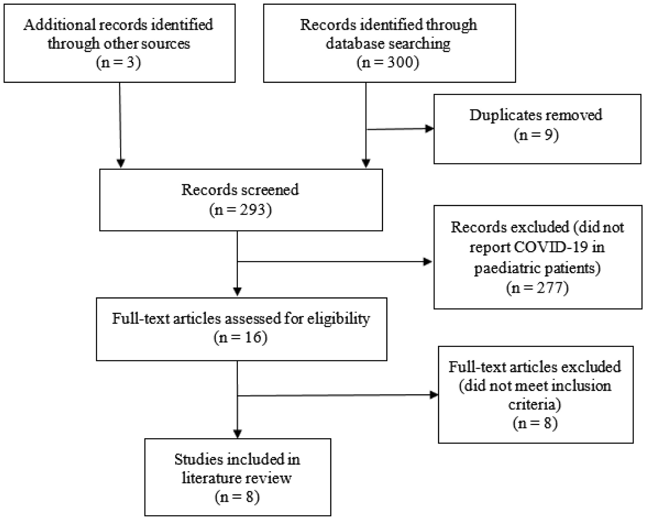
Moher D, Liberati A, Tetzlaff J, et al. (2009) Preferred reporting items for systematic reviews and meta-analyses: the PRISMA statement. BMJ 339: 332-336. doi: 10.1136/bmj.b2535
![]() |
[11] | Feng K, Yun YX, Wang XF, et al. (2020) Analysis of CT features of 15 Children with 2019 novel coronavirus infection. Chin J Contemp Pediatr 58: E007-E007. |
[12] | Wang D, Ju XL, Xie F, et al. (2020) Clinical analysis of 31 cases of 2019 novel coronavirus infection in children from six provinces (autonomous region) of northern China. Chin J Contemp Pediatr 58: E011. |
[13] | Cai J, Xu J, Lin D, et al. (2020) A Case Series of children with 2019 novel coronavirus infection: clinical and epidemiological features. Clin Inf Dis . |
[14] | Ji LN, Chao S, Wang YJ, et al. (2020) Clinical features of pediatric patients with COVID-19: a report of two family cluster cases. World J Pediatr 1-4. |
[15] | Hu Z, Song C, Xu C, et al. (2020) Clinical characteristics of 24 asymptomatic infections with COVID-19 screened among close contacts in Nanjing, China. Sci China Life Sci 1-6. |
[16] |
Xia W, Shao J, Guo Y, et al. (2020) Clinical and CT features in pediatric patients with COVID-19 infection: Different points from adults. Pediatric Pulmonol 55: 1169-1174. doi: 10.1002/ppul.24718
![]() |
[17] | Li W, Cui H, Li K, et al. (2020) Chest computed tomography in children with COVID-19 respiratory infection. Pediatric Radiol 1-4. |
[18] | StatistaNumber of novel coronavirus COVID-19 cumulative confirmed and death cases in China from January 20 to April 24, 2020.Available from: https://www.statista.com/statistics/1092918/china-wuhan-coronavirus-2019ncov-confirmed-and-deceased-number/. |
[19] | European Centre for Disease Prevention and Control (2020) Coronavirus disease 2019 (COVID-19) pandemic: increased transmission in the EU/EEA and the UK-seventh update. |
[20] |
Zhou P, Yang X, Wang X, et al. (2020) A pneumonia outbreak associated with a new coronavirus of probable bat origin. Nature 579: 270-273. doi: 10.1038/s41586-020-2012-7
![]() |
[21] |
Wrapp D, Wang N, Corbett KS, et al. (2020) Cryo-EM structure of the 2019-nCoV spike in the prefusion conformation. Science 367: 1260-1263. doi: 10.1126/science.abb2507
![]() |
[22] |
Chan JF, Yuan S, Kok K, et al. (2020) A familial cluster of pneumonia associated with the 2019 novel coronavirus indicating person-to-person transmission: a study of a family cluster. Lancet 395: 514-523. doi: 10.1016/S0140-6736(20)30154-9
![]() |
[23] | Sun K, Chen J, Viboud C (2020) Early epidemiological analysis of the coronavirus disease 2019 outbreak based on crowdsourced data: a population-level observational study. Lancet Digital Health . |
[24] | Lauer SA, Grantz KH, Bi Q, et al. (2020) The Incubation Period of Coronavirus Disease 2019 (COVID-19) From Publicly Reported Confirmed Cases: Estimation and Application. Ann Intern Med . |
[25] |
Virlogeux V, Fang VJ, Wu JT, et al. (2015) Incubation Period Duration and Severity of Clinical Disease Following Severe Acute Respiratory Syndrome Coronavirus Infection. Epidemiology 26: 666-669. doi: 10.1097/EDE.0000000000000339
![]() |
[26] |
Riou J, Althaus CL (2020) Pattern of early human-to-human transmission of Wuhan 2019 novel coronavirus (2019-nCoV), December 2019 to January 2020. Eurosurveillance 25. doi: 10.2807/1560-7917.ES.2020.25.4.2000058
![]() |
[27] |
Huang C, Wang Y, Li X, et al. (2020) Clinical features of patients infected with 2019 novel coronavirus in Wuhan, China. Lancet 395: 497-506. doi: 10.1016/S0140-6736(20)30183-5
![]() |
[28] | Yang Y, Yang M, Shen C, et al. (2020) Evaluating the accuracy of different respiratory specimens in the laboratory diagnosis and monitoring the viral shedding of 2019-nCoV infections. MedRxiv . |
[29] |
Li Y, Xia L (2020) Coronavirus Disease 2019 (COVID-19): Role of Chest CT in Diagnosis and Management. Am J Roentgenol 1-7. doi: 10.2214/AJR.19.22691
![]() |
[30] |
Calfee C, Matthay M, Kangelaris K, et al. (2015) Cigarette Smoke Exposure and the Acute Respiratory Distress Syndrome. Crit Care Med 43: 1790-1797. doi: 10.1097/CCM.0000000000001089
![]() |
1. | Xingyu Wang, Zhijun Liu, Lianwen Wang, Caihong Guo, Huili Xiang, An application of a novel geometric criterion to global-stability problems of a nonlinear SEIVS epidemic model, 2021, 1598-5865, 10.1007/s12190-020-01487-5 | |
2. | Gilberto González-Parra, Miguel Díaz-Rodríguez, Abraham J. Arenas, Optimization of the Controls against the Spread of Zika Virus in Populations, 2020, 8, 2079-3197, 76, 10.3390/computation8030076 | |
3. | Emile F. Doungmo Goufo, Yasir Khan, Qasim Ali Chaudhry, HIV and shifting epicenters for COVID-19, an alert for some countries, 2020, 139, 09600779, 110030, 10.1016/j.chaos.2020.110030 | |
4. | Sandeep Sharma, Fateh Singh, Backward bifurcation in a cholera model with a general treatment function, 2021, 3, 2523-3963, 10.1007/s42452-021-04189-0 | |
5. | Saif Ullah, Muhammad Farooq Khan, Syed Azhar Ali Shah, Muhammad Farooq, Muhammad Altaf Khan, Mustafa bin Mamat, Optimal control analysis of vector-host model with saturated treatment, 2020, 135, 2190-5444, 10.1140/epjp/s13360-020-00855-1 | |
6. | Harendra Pal Singh, Sumit Kaur Bhatia, Riya Jain, Yashika Bahri, 2021, Chapter 1, 978-981-16-1695-2, 1, 10.1007/978-981-16-1696-9_1 | |
7. | Thongchai Botmart, Qusain Hiader, Zulqurnain Sabir, Muhammad Asif Zahoor Raja, Wajaree Weera, Stochastic Investigations for the Fractional Vector-Host Diseased Based Saturated Function of Treatment Model, 2023, 74, 1546-2226, 559, 10.32604/cmc.2023.031871 | |
8. | Afeez Abidemi, Kolade M. Owolabi, Edson Pindza, Modelling the transmission dynamics of Lassa fever with nonlinear incidence rate and vertical transmission, 2022, 597, 03784371, 127259, 10.1016/j.physa.2022.127259 | |
9. | Fereshte Gazori, Mahmoud Hesaaraki, Three-dimensional spread analysis of a Dengue disease model with numerical season control, 2021, 14, 1793-5245, 10.1142/S1793524521500662 | |
10. | Xiaodan Wei, Xu Zhao, Wenshu Zhou, Global stability of a network-based SIS epidemic model with a saturated treatment function, 2022, 597, 03784371, 127295, 10.1016/j.physa.2022.127295 | |
11. | Shahram Rezapour, Joshua Kiddy K. Asamoah, Sina Etemad, Ali Akgül, İbrahim Avcı, Sayed M. El Din, On the fractal-fractional Mittag-Leffler model of a COVID-19 and Zika Co-infection, 2023, 55, 22113797, 107118, 10.1016/j.rinp.2023.107118 | |
12. | Harouna Ouedraogo, Ali Traoré, Global Properties of a Delayed Vector-borne Disease Model with Partial Protection of Susceptible Humans, 2023, 0971-3514, 10.1007/s12591-023-00652-z | |
13. | Ajimot Folashade Adebisi, Morufu Oyedunsi Olayiwola, Ibrahim Adeshola Adediran, Adedapo Ismaila Alaje, A Novel Mathematical Model and Homotopy Perturbation Method Analyzing the Effects of Saturated Incidence and Treatment Rate on COVID-19 Eradication, 2024, 48, 2731-8095, 625, 10.1007/s40995-024-01608-w | |
14. | Xiaodan Wei, Global analysis of a network-based SIR epidemic model with a saturated treatment function, 2024, 17, 1793-5245, 10.1142/S1793524523501127 | |
15. | Tanuja Das, Prashant K. Srivastava, Stability and codimension 2 bifurcations in an SIR model with incubation delay, 2024, 79, 14681218, 104127, 10.1016/j.nonrwa.2024.104127 | |
16. | Junmei Liu, Yonggang Ma, Optimal control analysis of COVID-19 stochastic model with comprehensive strategies, 2024, 12, 2164-2583, 10.1080/21642583.2024.2350171 | |
17. | Prakash Raj Murugadoss, Venkatesh Ambalarajan, Vinoth Sivakumar, Prasantha Bharathi Dhandapani, Dumitru Baleanu, Analysis of Dengue Transmission Dynamic Model by Stability and Hopf Bifurcation with Two-Time Delays, 2023, 28, 2768-6701, 10.31083/j.fbl2806117 | |
18. | S. Jothika, M. Radhakrishnan, Stability and Control of a Vector-Host Disease Model with Time Delay and Saturated Treatment, 2025, 19, 1823-8343, 177, 10.47836/mjms.19.1.10 | |
19. | Tapan Sarkar, Pankaj Biswas, Prashant K. Srivastava, Modeling the effects of media information and saturated treatment on malaria disease with NSFD method, 2025, 18, 1793-5245, 10.1142/S1793524524500013 |
Notation | Value | |
Λh | 0.0002/day | |
c | 0.0002/day | |
β1 | 0.000044 /day | |
α1 | 0.003 /day | |
μh | 0.00020 /day | |
b | 0.4/day | |
δh | 0.002 /day | |
γ | 0.1/day | |
Λv | 0.08/day | |
β2 | 0.007 /day | |
α2 | 0.02/day | |
μv | 0.2/day | |
bo | 0.01/day |