Loading [MathJax]/jax/output/SVG/jax.js
Review Special Issues

Improving microplastic research

  • There has been a virtual explosion of research on microplastics. Every week new articles are published in scientific journals. However, not all of them are original or important. Dozens of papers come out monthly that report the number of microplastic particles found in some water body, but they cannot be compared because there are no standardized methods for collection or analysis. However, it has become clear that collecting microplastics with nets misses most of the microplastics, since microfibers, which are by far the most abundant type when whole water samples are analyzed, pass through nets. These microfibers are derived primarily from synthetic clothing via wastewater from washing machines. Another common study documents that some species consumes microplastics. It seems that every animal studied eats them; it would be of greater interest to find one that does not ingest them. Although animals consume them, few studies have examined how soon and how many are egested. Most may pass through the gut without causing any noticeable effects. This is an important area to study. Microplastics are considered vectors for transferring contaminants to animals and up the food chain, but few studies demonstrate this with realistic scenarios such as providing the animals some “real” food and time to egest. Effects attributed to microplastics may be symptoms of inadequate nutrition or a clogged digestive tract. It is also important to learn how much of the adsorbed contaminants the gut can desorb during the time that microplastics are passing through. Future feeding studies should not use spherical microplastics which are rare in aquatic environments but should use primarily microfibers which are the predominant shape found, provide real food, and allow time for egestion to occur. Other research needs include additional studies on soil and terrestrial biota and developing ways to modify the manufacture of textiles to shed fewer microfibers.

    Citation: Judith S. Weis. Improving microplastic research[J]. AIMS Environmental Science, 2019, 6(5): 326-340. doi: 10.3934/environsci.2019.5.326

    Related Papers:

    [1] Manal M. Yousef, Rehab Alsultan, Said G. Nassr . Parametric inference on partially accelerated life testing for the inverted Kumaraswamy distribution based on Type-II progressive censoring data. Mathematical Biosciences and Engineering, 2023, 20(2): 1674-1694. doi: 10.3934/mbe.2023076
    [2] Lernik Asserian, Susan E. Luczak, I. G. Rosen . Computation of nonparametric, mixed effects, maximum likelihood, biosensor data based-estimators for the distributions of random parameters in an abstract parabolic model for the transdermal transport of alcohol. Mathematical Biosciences and Engineering, 2023, 20(11): 20345-20377. doi: 10.3934/mbe.2023900
    [3] Hiroshi Nishiura, Seiko Fujiwara, Akifumi Imamura, Takuma Shirasaka . HIV incidence before and during the COVID-19 pandemic in Japan. Mathematical Biosciences and Engineering, 2024, 21(4): 4874-4885. doi: 10.3934/mbe.2024215
    [4] M. G. M. Ghazal, H. M. M. Radwan . A reduced distribution of the modified Weibull distribution and its applications to medical and engineering data. Mathematical Biosciences and Engineering, 2022, 19(12): 13193-13213. doi: 10.3934/mbe.2022617
    [5] M. Nagy, Adel Fahad Alrasheedi . The lifetime analysis of the Weibull model based on Generalized Type-I progressive hybrid censoring schemes. Mathematical Biosciences and Engineering, 2022, 19(3): 2330-2354. doi: 10.3934/mbe.2022108
    [6] Saralees Nadarajah . Remark on the Paper by Rao And Kakehashi (2005). Mathematical Biosciences and Engineering, 2006, 3(2): 385-387. doi: 10.3934/mbe.2006.3.385
    [7] Cruz Vargas-De-León . Global analysis of a delayed vector-bias model for malaria transmission with incubation period in mosquitoes. Mathematical Biosciences and Engineering, 2012, 9(1): 165-174. doi: 10.3934/mbe.2012.9.165
    [8] Rashad A. R. Bantan, Zubair Ahmad, Faridoon Khan, Mohammed Elgarhy, Zahra Almaspoor, G. G. Hamedani, Mahmoud El-Morshedy, Ahmed M. Gemeay . Predictive modeling of the COVID-19 data using a new version of the flexible Weibull model and machine learning techniques. Mathematical Biosciences and Engineering, 2023, 20(2): 2847-2873. doi: 10.3934/mbe.2023134
    [9] Helong Liu, Xinyu Song . Stationary distribution and extinction of a stochastic HIV/AIDS model with nonlinear incidence rate. Mathematical Biosciences and Engineering, 2024, 21(1): 1650-1671. doi: 10.3934/mbe.2024072
    [10] Said G. Nassr, Amal S. Hassan, Rehab Alsultan, Ahmed R. El-Saeed . Acceptance sampling plans for the three-parameter inverted Topp–Leone model. Mathematical Biosciences and Engineering, 2022, 19(12): 13628-13659. doi: 10.3934/mbe.2022636
  • There has been a virtual explosion of research on microplastics. Every week new articles are published in scientific journals. However, not all of them are original or important. Dozens of papers come out monthly that report the number of microplastic particles found in some water body, but they cannot be compared because there are no standardized methods for collection or analysis. However, it has become clear that collecting microplastics with nets misses most of the microplastics, since microfibers, which are by far the most abundant type when whole water samples are analyzed, pass through nets. These microfibers are derived primarily from synthetic clothing via wastewater from washing machines. Another common study documents that some species consumes microplastics. It seems that every animal studied eats them; it would be of greater interest to find one that does not ingest them. Although animals consume them, few studies have examined how soon and how many are egested. Most may pass through the gut without causing any noticeable effects. This is an important area to study. Microplastics are considered vectors for transferring contaminants to animals and up the food chain, but few studies demonstrate this with realistic scenarios such as providing the animals some “real” food and time to egest. Effects attributed to microplastics may be symptoms of inadequate nutrition or a clogged digestive tract. It is also important to learn how much of the adsorbed contaminants the gut can desorb during the time that microplastics are passing through. Future feeding studies should not use spherical microplastics which are rare in aquatic environments but should use primarily microfibers which are the predominant shape found, provide real food, and allow time for egestion to occur. Other research needs include additional studies on soil and terrestrial biota and developing ways to modify the manufacture of textiles to shed fewer microfibers.


    Since Kauffman introduced a binary network called Boolean network (BN) to study the evolution behavior in genetic regulatory networks (GRNs) [1], it has garnered considerable interest from biologists, systems scientists, and others. In a BN, variables are used to represent genes with values of 1 or 0, where 1 implies that the gene is active, and 0 implies that the gene is inactive. When there are external disturbances regulations, BNs are naturally extended to BCNs. In addition, probabilistic Boolean networks (PBNs) and switching Boolean networks (SBNs) are investigated due to the switching and random phenomena in GRNs [2,3].

    In fact, BNs (BCNs) with logical function forms are nonlinear networks. Thus, traditional discrete-time linear system theory cannot be used to investigate research problems. Cheng et al. [4] invented the semi-tensor product (STP) of matrices to convert the logical dynamical system into a typical discrete-time linear system. Some methods and ideas in linear system theory can be applied to BNs (BCNs) by using the STP, which further helps scientists analyze and control GRNs for disease intervention [5] or work on feedback shift registers [6] and so on [7,8,9]. Since then, various properties of BNs have been investigated, such as controllability, observability, stabilization and so on [10,11,12,13,14,15,16,17,18,19,20]. Furthermore, as a helpful tool, the STP method also is used in hybrid dynamic systems and fuzzy systems [21,22,23,24,25,26].

    In the practical GRNs, the state evolution is complicated and the measuring equipment has limitation [27]. Therefore, it is an effective solution for scientists to measure the output and render the system output to track the desired signals to help study the system's dynamics. It is also of great significance in the application of robots and flight control [28,29,30]. By reviewing the literature, we obtain that the current studies on output tracking issues of BCNs can be mainly divided into the two following categories according to the objectives of output tracking: track a constant reference signal and track a time-varying reference trajectory [27,31,32,33,34,35]. Methods for designing the state feedback control law were described in [27] to let the system's output track a constant reference signal stably after a finite time. In [31], the switching sequence is found by combining the method of set stabilization, so that the SBNs can track a given a given constant reference signal. [32] constructed an auxiliary system to help the outputs of a BCN track the outputs of a reference system. Since it may cost a lot to control over an infinite horizon, [33] considered tracking a given reference output trajectory. In summary, the output tracking problem is an inevitable and crucial issue for GRNs.

    In addition, the output tracking problem has other practical significance. For example, the motion of ships carrying heavy cargo needs to track a desired line reserved before, thereby minimizing financial burden [36]. Furthermore, considering that the output tracking research might help control the spread of future epidemics, we mainly care about tracking a given finite length of time-varying reference output trajectory. Moreover, the idea of adding controls to the output is motivated by the research problem investigated in [37]. In the study of a functional system related to avalanche warning, context-alert of context model combined with terrain temperature, snow height, and accelerometer as the total input variables has a specific effect on the output of functional system [37]. Hence, we add controls to the system output to describe these system models. It is worth highlighting that the authors in [33] studied the output tracking problem of BCNs. Nonetheless, the method in [33] fails to solve the problem in some cases. To our knowledge, no study has been done considering the controls in the output to solve the output tracking problem. The system considered in this paper has controls in both state transition and output models. Therefore, to a certain extent, the method discussed in this paper can realize the output tracking problem that cannot be realized in [33]. In the following, we highlight the main contributions of this paper:

    ● From the perspectives of set and matrix, for the BCN system with output having controls, we give some equivalent conditions to solve the reference trajectory output tracking issue.

    ● Based on the obtained theorem, the authors construct an algorithm to determine whether the output tracking issue is solvable.

    ● If the problem can be solved, we develop an algorithm to obtain a feasible control sequence, allowing the system to track the reference output trajectory in a finite range.

    The main structure of this paper is as follows. We introduce the preliminaries in Section 2. The main theorems for the solvability of output tracking issues are obtained in Section 3. Finally, some biological examples are proposed to verify our results in Section 4. A concise conclusion is shown in Section 5.

    First, for the convenience of subsequent description, some basic notations are given here.

    D:={0,1}, real numbers are denoted by R and the set of positive integers is denoted by Z+.

    Δq:={δiq|1iq}, where δiq represents an q-dimensional column vector with the ith element being 1 and others are 0.

    ● The ith column and ith row of matrix Q are denoted by Coli(Q) and Rowi(Q), respectively.

    ● We call a matrix QMm×n logical matrix, if each column vector of it has only one element 1, and the other elements are 0. In this paper, denote the set of m×n-dimensional logical matrices by Lm×n. Besides, Bm×n denotes the set of m×n Boolean matrices, with all elements taking value from D.

    ● For a logical matrix A=[δi1mδi2mδinm], its abbreviation is A=δm[i1i2in].

    [ϵ,ξ]:={ϵ,ϵ+1,ϵ+2,,ξ}, where ϵ,ξZ+.

    1k or 0k is the k-dimensional column vector whose elements are all equal to 1 or 0, respectively.

    ● If α(t)=m1δi12n+m2δi22n++mkδik2n, where m1,m2,,mkZ+, Ξ(α(t)):={δi12n,δi22n,,δik2n}. On the contrary, if one set Ω={δi12n,δi22n,,δik2n}, then Ψ(Ω):=kj=1δij2n. To describe concisely, denote Ψ(Ω)=δi1,i2,,ik2n.

    ● For two vectors ρ=[ρ1ρ2ρs]Rs, σ=[σ1σ2σs]Rs. We denote the element-wise multiplication of them by

    ρσ:=[ρ1σ1ρ2σ2ρsσs].

    In this section, we introduce the definition of the STP and how to transform BNs from logical expressions to algebraic forms.

    Definition 2.1. [4] For two matrices PMa×b and QMc×d, the semi-tensor product of them is defined by

    PQ=(PIl/b)(QIl/c),

    where l=lcm(b,c) is the least common multiple of b and c, and is the Kronecker product.

    When b=c, the STP of matrix is consistent with ordinary matrix multiplication. In this article, we will omit "" without affecting the results to facilitate reading.

    Before using the STP to obtain the algebraic expression of BCNs, we show equivalence between Boolean variables and their vector forms. Here, 1 is equivalent to δ12 and 0 is equivalent to δ22.

    Lemma 2.1. [4] For a logical function g(x1,,xn):DnD, after changing all arguments xi to their vector form xi, i.e., xiΔ2, i[1,n], it has an equivalent algebraic form g(x1,,xn)=Lgx1xn, where the structure matrix LgL2×2n can be uniquely determined by g.

    Consider the logical representation of a BCN is abbreviated as

    xi(t+1)=gi(u1(t),,um(t),x1(t),,xn(t)), (2.1)

    with its output system being

    yj(t)=hj(u1(t),,um(t),x1(t),,xn(t)), (2.2)

    where xi(t),uk(t),yj(t)D, i[1,n], k[1,m], j[1,p] are logical variables. gi:Dm+nD,i[1,n], hj:Dm+nD,j[1,p] are logical functions. Then, after changing the logical form of variables to the vector form, we define x(t)=ni=1xi(t)Δ2n,u(t)=mk=1uk(t)Δ2m. According to Lemma 2.1, we can transform equation (2.1) into

    xi(t+1)=Miu(t)x(t), (2.3)

    where structure matrices are specified as MiL2×2m+n,i[1,n]. Likewise, define y(t)=pj=1yj(t). Then the outputs are

    yj(t+1)=Nju(t)x(t), (2.4)

    where NjL2×2m+n,j[1,p]. Therefore, we can determine the algebraic form of BCN (2.1) and its output (2.2) as

    {x(t+1)=Lu(t)x(t),y(t)=Hu(t)x(t), (2.5)

    where L, which can be obtained by L=M1M2Mn, is referred to as the network transition matrix. Similarly, H is called an output matrix which can be expressed as H=N1N2Np, where "" is the Khatri-Rao product of matrices.

    Remark 2.1. Without the loss of generality, in the equations (2.1) and (2.2), the evolution of the state and the output, respectively, in the BCN model we give, is related to the same control sequence. If the state and output are affected by different control variables, we can still combine all the control variables with a dummy matrix [4]. Then, it will make the control sequences the same and larger dimensional than before for the convenience of subsequent studies.

    Based on the above STP work, we can analyze the algebraic form of BCNs to study the output tracking issue. For simplicity, denote a control sequence ut by ut={u(0),u(1),,u(t)}. Thus, the output of the system (2.5) under ut is shown as y(t,x(0),ut). Then, there is y(t,x(0),ut)=Hu(t)Lu(t1)Lu(t2)Lu(0)x(0). Since we are investigating the problem of reference trajectory output tracking, there needs to be an assigned reference output trajectory yP:

    yo(1)=δy12p,yo(2)=δy22p,,yo(P)=δyP2p.

    Next, we will give the definition of reference trajectory output tracking and the solvable conditions for the output tracking issue will be discovered using the properties of BCNs.

    Definition 3.1. [33] Consider BCN (2.5) with a given initial state x(0) and a reference output trajectory yP. The (reference trajectory) output tracking issue is solvable, if we can find a control sequence uP such that y(t;x(0),ut)=yo(t),t[1,P].

    We first regard u(t)x(t) in (2.5) as a control-state pair. For convenience of subsequent description, let u(t)=δkt2m, x(t)=δit2n. Then u(t)x(t)=δjt2m+n, where jt=2n(kt1)+it. For the output yo(t)=δyt2p, the set of u(t)x(t) that can realize output tracking is

    Ω(t)={u(t)x(t)=δjt2m+n|Coljt(H)=δyt2p},t[1,P].

    We construct sets X(t),Λ(t) and Γ(t) alternatively as shown below to address the output tracking issue, where t[1,P].

    First, the state set obtained from state x(0) through one step is X(1)={x(1)|x(1)=Lu(0)x(0),u(0)Δ2m}. Define the set Λ(t)={˜u(t)x(t),˜u(t)Δ2m,x(t)X(t)},t[1,P]. Γ(t) represents the intersection of Λ(t) and Ω(t), i.e.,

    Γ(t)=Λ(t)Ω(t),t[1,P]. (3.1)

    It is essential to mention that for t[2,P]

    X(t)={x(t)|x(t)=Lu(t1)x(t1),u(t1)x(t1)Γ(t1)}. (3.2)

    Remark 3.1. Ω(t) is the control-state pairs set whose elements can produce the desired output according to H. X(t) is the state set under control sequence which meets the condition of tracking, from the perspective of network transition matrix L of dynamical equation. To unify the dimensions of the two sets, we define the set Λ(t).

    Following the definition of sets X(t),Λ(t) and Γ(t), a theorem can be obtained to determine the solvability of the output tracking issue from the perspective of the set.

    Theorem 3.1. Given an initial state x(0)=δi02n, a positive integer P and a reference output trajectory yP, the output tracking issue of BCN (2.5) is solvable if and only if

    Γ(P).

    Proof. (Sufficiency) For any t[1,P1], if Γ(t)=, by calculation it has X(t+1)={x(t+1)|x(t+1)=Lu(t)x(t),u(t)x(t)Γ(t)}=. Similarly, it can be obtained that for any t[t+1,P], X(t)={x(t)|x(t)=Lu(t1)x(t1)}= always holds. It shows that Λ(t)= and Γ(t)=, which is in contradiction to Γ(P). Therefore, the condition Γ(P) implies that Γ(t),t[1,P]. Then, we can choose a u(P)x(P)Γ(P) and denote them by u(P)=δkP2m,x(P)=δiP2n, respectively. Since x(P)X(P), there exists u(P1)x(P1)Γ(P1), where u(P1)=δkP12m,x(P)=δiP12n, such that Lu(P1)x(P1)=x(P)=δiP2n holds. Similarly, we can find a series of control-state pairs {u(1)x(1),u(2)x(2),,u(P)x(P)}, which satisfies u(t)x(t)Γ(t) and Lu(t)x(t)=x(t+1),t[1,P1]. In addition, for x(0)=δi02n, we only need to determine u(0)=δk02m so that Lu(0)x(0)=x(1). Hence, there exists a control sequence uP={u(0)=δk02m,u(1)=δk12m,,u(P)=δkP2m} such that for any t[1,P], u(t)x(t)Γ(t), then y(t;x(0),ut)=yo(t) holds. Thus, the solvable goal can be achieved.

    (Necessity) If Γ(P)=, based on (3.1), we have Λ(P)Ω(P)=. Then, for any x(P)X(P), ˜u(P)x(P) constructed by ˜u(P)Δ2m does not belong to Ω(P). Therefore, y(P)=H˜u(P)x(P)yo(P), which breaks the requirement that the output tracking issue of BCN (2.5) is solvable.

    Theorem 3.1 shows that t[1,P], Γ(t) means that there exists u(t)x(t) satisfying both dynamical update condition and output tracking condition. It determines that the output tracking goal of BCN (2.5) can be achieved from the perspective of the set. Next, we consider giving another theorem to realize the goal through vector expression from the perspective of matrix calculation.

    Denote

    w(t)=Ψ(Ω(t))B2m+n×1, (3.3)

    which is the vector form of the set Ω(t) including all the control-state pairs that can produce output yo(t). Define

    γ(t)=w(t)(12mLγ(t1)),t[1,P], (3.4)

    with γ(0):=12mx(0). Then, we have the following necessary and sufficient criterion for output tracking using vector expression.

    Theorem 3.2. Given an initial state x(0)=δi02n and a positive integer P, the output tracking issue of BCN (2.5) is solvable if and only if γ(P)002m+n.

    Proof. For sufficiency, if there is t1[1,P1], such that γ(t1)=02m+n, then by (3.4), the equation γ(t)=02m+n,t[t1+1,P] holds, which is in contradiction with the condition γ(P)02m+n. Thus, it concludes that γ(t)02m+n,t[1,P]. For γ(P)02m+n, we can take u(P)x(P)=δjP2m+nΞ(γ(P)), and denote them by u(P)=δkP2m,x(P)=δiP2n, respectively. According to the construction of γ(t) in (3.4), it implies that y(P)=Hu(P)x(P)=yo(P). Then, we can choose u(t1)x(t1)Ξ(γ(t1)) satisfying that Lu(t1)x(t1)=x(t)=δit2n, where u(t1)=δkt12m,x(t1)=δit12n,t=P,P1,,2. It also holds that y(t)=Hu(t)x(t)=yo(t). For t=1, u(0) is determined by satisfying Lu(0)x(0)=x(1)=δi12n. Hence, there is a uP={u(0)=δk02m,u(1)=δk12m,,u(P)=δkP2m} so that t[1,P], y(t;x(0),ut)=yo(t) holds, which means that there is one way that the output tracking goal of BCN (2.5) can be resolved. As for necessity, it is removed here since it is analogous to Theorem 3.1.

    Theorem 3.1 gives the necessary and sufficient conditions for the solvability of output tracking problem from the set viewpoint, which helps us to understand. In Theorem 3.2, the criterion is given by vector method, which is convenient for practical calculation and judgment. Then, Algorithm 1 is given below to illustrate the general steps for determining whether the output tracking issue can be solved.

    Algorithm 1 Determine the solvability of output tracking issue.
    Input: x(0)=δi02n, P, and the reference output trajectory yP with a known BCN (2.5)
    1: Initialize γ(0)=12mδi02n, t=1.
    2: while t=1,,P do
    3:   Calculate the corresponding Ω(t) and w(t) based on yo(t)=δyt2p.
    4:   Calculate γ(t)=w(t)(12mLγ(t1)).
    5:  if γ(t)=02m+n then
    6:   the output tracking issue is unsolvable.
    7:  else
    8:  tt+1.
    9:  end if
    10: else
    11:   the output tracking issue of BCN (2.5) is solvable.
    12: end while

    After we investigate whether the output tracking issue for a reference trajectory in a given finite time can be solved, we consider finding a control sequence satisfying the condition that BCN (2.5) is solvable, such that the outputs can achieve the given reference output trajectory.

    The basic idea to solve the problem is to calculate u(t) and x(t) backward by γ(t), t[1,P]. Obviously, the control-state pairs that can realize output tracking may be not unique at each time, and our goal is to find a feasible control sequence so that the output trajectory can track the reference output trajectory. Algorithm 2 gives the design method of the controllers.

    Algorithm 2 Get a feasible control sequence {u(0),u(1),,u(P)}, such that BCN (2.5) realize the output tracking.
    Input: x(0)=δi02n, P, and the reference output trajectory yP with a known BCN (2.5)
    1: Determine that whether the problem can be solved according to Algorithm 1.
    2: if it is solvable then
    3:   Randomly choose u(P)x(P)=δjP2m+nΞ(γ(P)), and denote them by u(P)=δkP2m,x(P)=δiP2n.
    4:   while t=P,P1,,1 do
    5:     Choose u(t1)x(t1)Ξ(γ(t1)) satisfying that Lu(t1)x(t1)=x(t)=δit2n. Denote u(t1)=δkt12m,x(t1)=δit12n.
    6:     tt1
    7:   end while
    8:   Select u(0)=δk02m, which satisfies Lu(0)x(0)=x(1).
    9: else end

    Remark 3.2. It is worth to note that Algorithm 2 is based on the Algorithm 1. We need to calculate all γ(t), t[1,P] and determine that γ(P)02m+n. Therefore, Step 3 in Algorithm 2 is a way to select the feasible control u and x. Finally, the control sequence that can achieve the output tracking is determined based on the γ(t), t[1,P], calculated in Algorithm 1.

    Furthermore, it has been proved that solving control problems of BCNs using the STP is an NP-hard problem and causes exponential computational burden. In particular, the worst-case computational complexity involved in determining the problem's solvability (Algorithm 1) is O(2nP), and designing the control sequence (Algorithm 2) is O(2n+mP).

    Proposition 3.1. Given x(0)=δi02n, under the control sequence {u(0),u(1),,u(P)} obtained in Algorithm 2, the state trajectory {x(1)=δi12n,x(2)=δi22n,,x(P)=δiP2n} will produce the desired reference output trajectory yP.

    Proof. From Algorithm 2, we can find that

    x(t)={Lu(0)x(0)t=1,Lu(t1)x(t1)t[2,P]. (3.5)

    For any t[1,P], there is

    y(t)=Hu(t)x(t)=Hu(t)Lu(t1)x(t1)=Hu(t)Lu(t1)Lu(t2)Lu(1)Lu(0)x(0).

    Since u(t)x(t)Ξ(γ(t)) holds for all t[1,P], it implies that u(t)x(t)Ω(t). Therefore, it can be obtained that y(t)=yo(t),t[1,P].

    In daily life, constraints are everywhere. Taking the treatment of patients by doctors as an example, the state of patients or cells can be regarded as the state of the system, and the prescription drugs issued by doctors can be regarded as the control of the system. The purpose of doctors' treatment of patients is to hope that patients will enter a continuous healthy state, so some unhealthy and sick states should be avoided [38]. In some cases, the type of drugs will be determined according to the state of the patient. For example, when the patient is in the state of drinking alcohol, the doctor will not consider taking cephalosporin anti-inflammatory drugs, which is the transition constraint considered here [39]. In addition, if some drugs were developed a long time ago, and with the increase of medical level, we find the use of these drugs may have undesirable side effects on the human body, then doctors will not consider prescribing these types of drugs. For example, furazolidone as an effective drug, is usually used to treat gastrointestinal diseases such as dysentery and enteritis caused by bacteria and protozoa. However, scientists found that it has potentially carcinogenic properties [40]. Hence, doctors won't use compound preparation containing furazolidone now, and it can be one of the examples for the input control constraints. Therefore, in controllers' design, we should also consider changes in state, transition and input constraints.

    (1) State constraint

    When solving the output tracking issue of the system and designing the controllers, if a state x(t)=δi2n should be avoided, then the ith row of matrix L should be

    Rowi(L)=02m+n.

    At this point, we do not consider any transition from other states to x(t)=δi2n.

    (2) Transition constraint

    In a BCN, a transition constraint forbids the control input u(t) for a state x(t). For example, if the transition from the state x(t)=δi2n using control input u(t)=δk2m is forbidden, then we have

    Col2n(k1)+i(L)=02n,andCol2n(k1)+i(H)=02p.

    (3) Input constraint

    The input constraint means there are some controls that we cannot take. Suppose that u(t)=δk2m has to be forbidden, then the k-th block of L and H will be null matrices, that is

    Lk:=Lδk2m=02n×2n,andHk:=Hδk2m=02p×2n.

    Example 4.1. Consider BCN in [33]:

    {x1(t+1)=¬u1(t)(x2(t)x3(t)),x2(t+1)=¬u1(t)u2(t)x1(t),x3(t+1)=¬u1(t)(u2(t)(u3(t)x1(t))),y1(t)=(u1(t)u3(t))(¬u1(t)u2(t))x1(t),y2(t)=(¬u1(t)u2(t))(u2(t)u3(t))x2(t). (4.1)

    This is a simplified BCN model of lac operon in Escherichiacoli. Applying the STP method, the following algebraic form can be obtained:

    {x(t+1)=Lu(t)x(t),y(t)=Hu(t)x(t), (4.2)

    where x(t)=3i=1xi(t)Δ8, u(t)=3k=1uk(t)Δ8, y(t)=2j=1yj(t)Δ4. Besides, the network transition matrix and the output matrix are

    L=δ8[88888888|8888888888888888|8888888811153337|1115333733374448|44484448],
    H=δ4[11111111|1111333322222222|2222444411111111|1111111111113333|11113333].

    At the beginning, we assume that x(0)=δ28, and give two reference output trajectories as:

    Table 1.  Output trajectory 1.
    t 1 2 3 4
    yo1 1 0 0 0
    yo2 0 1 0 0
    yo δ24 δ34 δ44 δ44

     | Show Table
    DownLoad: CSV
    Table 2.  Output trajectory 2.
    t 1 2 3 4
    yo1 0 1 0 0
    yo2 1 0 0 0
    yo δ34 δ24 δ44 δ44

     | Show Table
    DownLoad: CSV

    To better simulate the GRNs, we assume that there are three types of constraints in (4.2):

    (1) State constraint: State δ18 should be avoided, which means that Row1(L)=0064.

    (2) Transition constraint: For state x(t)=δ68, it is prohibited to use control input u(t)=δ38. Then, the two matrices become L3=δ8[88888088], H3=δ4[22222022]. With a slight abuse of notation, we use δ0i here to represent 00i.

    (3) Input constraint: Considering the specification about the concentration of extra cellular lactose, the control input u=3k=1uk=δ28 and u=3k=1uk=δ68 are forbidden. Then, we have L2=L6=008×8, H2=H6=004×8.

    Under the three types of constraints, the new matrices are expressed as

    ˆL=δ8[88888888|0000000088888088|8888888800053337|0000000033374448|44484448],
    ˆH=δ4[11111111|0000000022222022|2222444411111111|0000000011113333|11113333].

    The following is to determine whether the output tracking issue can be solved for the given output trajectories 1 and 2. If it is solvable, we can give the corresponding controllers' design. Initialize γ(0)=118δ28, and it has γ(0)=δ2,10,18,26,34,42,50,5864 by calculation.

    We first consider whether the system can track the specified reference output trajectory 1.

    (1) For yo(1)=δ24, according to ˆH, we can get Ω(1)={δ1764,δ1864,δ1964,δ2064,δ2164,δ2364,δ2464,δ2564,δ2664,δ2764,δ2864} and w(1)=δ17,18,19,20,21,23,24,25,26,27,2864. Then, we have

    γ(1)=w(1)(112mˆLγ(0))=δ19,20,27,2864+3δ2464.

    (2) For yo(2)=δ34, we have Ω(2)={δ5364,δ5464,δ5564,δ5664,δ6164,δ6264,δ6364,δ6464} and w(2)=δ53,54,55,56,61,62,63,6464. Then, it holds that

    γ(2)=w(2)(12mˆLγ(1))=7δ56,6464.

    (3) For yo(3)=yo(4)=δ44, it holds that Ω(3)=Ω(4)={δ2964,δ3064,δ3164,δ3264}, and w(3)=w(4)=δ29,30,31,3264. Furthermore, we have

    γ(3)=w(3)(112mˆLγ(2))=14δ3264,
    γ(4)=w(4)(112mˆLγ(3))=14δ3264.

    It can be concluded that the output tracking issue of the system is solvable for reference output trajectory 1 since γ(4)008. Then, we can use the method in Algorithm 2 to find a feasible control sequence to realize output tracking for the output trajectory 1. The specific process is as follows. First, since P=4 and γ(4)=14δ3264, we can only get that u(4)x(4)=δ3264Ξ(γ(4)). Hence, by decomposition, we have u(4)=δ48 and x(4)=δ88. Next, we need to choose u(3)x(3)Ξ(γ(3)), satisfying ˆLu(3)x(3)=x(4)=δ88. Then, we have u(3)x(3)=δ3264 with u(3)=δ48 and x(3)=δ88. Similarly, we can obtain a control input sequence that meets the output tracking condition represented by {u(0)=δ18,u(1)=δ38,u(2)=δ78,u(3)=δ48,u(4)=δ48}, with corresponding state sequence denoted by {x(0)=δ28,x(1)=δ88,x(2)=δ88,x(3)=δ88,x(4)=δ88}. Note that this is only a feasible situation we have proposed, and it is not unique.

    Analogously, for reference output trajectory 2, we can obtain that

    γ(1)=3δ56,6464,γ(2)=6δ2464,γ(3)=6δ3264,γ(4)=6δ3264.

    It determines that the system can track reference output trajectory 2 since γ(4)008. Furthermore, the input sequence that meets the output tracking condition can be {u(0)=δ18,u(1)=δ78,u(2)=δ38,u(3)=δ48,u(4)=δ48}.

    In [33], there does not have any control in the output system. The system can realize output tracking under output trajectory 1, but fails under output trajectory 2. As one of the innovations of this paper, we add control input to the output system. We can find in this example that it makes the system realize output tracking under two reference output trajectories.

    Example 4.2. Consider a modified lactose operon model in Escherichia coli with 5 nodes [41]:

    {x1(t+1)=x3(t)u1(t),x2(t+1)=x1(t),x3(t+1)=x3(t)(x4(t)x2(t)),x4(t+1)=x5(t)(x4(t)¬x2(t)),x5(t+1)=x1(t)u2(t),y1(t)=x1(t)u1(t),y2(t)=x2(t)u2(t). (4.3)

    Based on the STP method, we can transfer the model to the form as (2.5) with x(t)=5i=1xi(t)Δ32, u(t)=2k=1uk(t)Δ4, y(t)=2j=1yj(t)Δ4, where L=δ32[1313171921232626262830303032] and H=δ4[1111111144444444]. Next, we suppose that there are some constraints:

    (1) State constraint: State δ3232 is avoided and Row32(L)=00128.

    (2) Transition constraint: For state x(t)=δ332, the control input u(t)=δ14 is limited, so we will have Col3(L)=0032,andCol3(H)=004.

    (3) Input constraint: Suppose that the control input u=2k=1uk=δ24 is forbidden. Finally, the matrices are changed to ˆL=δ32[130317192123262626283030300] and ˆH=δ4[1101111144444444].

    Here, we are going to check under the condition that the initial state is x(0)=δ2032, whether the output tracking issue can be solvable with the given output trajectory yo(1)=δ14,yo(2)=δ24,yo(3)=δ14. First, according to Algorithm 1, it has γ(0)=114δ2032=δ20,52,84,116128. Then, calculated by the while loop, we can obtain γ(1)=δ11,27,28,43,59,60,75,91,92,107,123,124128,γ(2)=δ105,107128,γ(3)=2δ17128. It shows that the output tracking issue of BCN (4.3) is solvable. Hence, we can use Algorithm 2 to get a feasible control sequence such that BCN (4.3) achieves output tracking.

    First of all, because of γ(P)=γ(3)=2δ17128, it can be divided to u(3)x(3)=δ14δ1732. Then, we aim to choose u(2)x(2)Ξ(γ(2)) such that ˆLu(2)x(2)=x(3)=δ1732. By calculation, it obtains u(2)=δ44,x(2)=δ932. Furthermore, we can get u(1)=δ14,x(1)=δ2732 and u(0)=δ34. Therefore, using the control sequence {u(0)=δ34,u(1)=δ14,u(2)=δ44,u(3)=δ14}, the output tracking issue based on the given reference trajectory can be solved.

    By using the STP, for the BCNs with controls in output, the reference trajectory output tracking issue is investigated. Some results to solve the output tracking issue are proposed and an algorithm is designed to judge the solvability. Moreover, the controllers' design algorithm is given by calculation when we have determined that the output tracking issue is solvable. To better apply the results to daily life, the corresponding changes in the network transition matrix and output matrix under some constraints simulated from reality are considered. In the end, the effectiveness of our results is shown by some examples. An important direction for future research is to investigate output tracking problem by reinforcement learning method. In addition, we can study the problems considered in this paper in BNs with time delay or switching signal.

    This work was jointly supported by the Natural Science Foundation of Zhejiang Province of China under Grant Nos. LR20F030001 and LD19A010001, and the National Natural Science Foundation of China under Grant 62173308.

    The authors declare that they have no known competing financial interests or personal relationships that could have appeared to influence the work reported in this paper.


    [1] Courtene-Jones W, Quinn B, Gary S, et al. (2017) Microplastic pollution identified in deep-sea water and ingested by benthic invertebrates in the Rockasll Trough, North Atlantic Ocean. Environ Poll 231: 271–280. doi: 10.1016/j.envpol.2017.08.026
    [2] Sanchez-Vidal A, Thompson R, Canala M, et al. (2018) The imprint of microfibres in Southern European deep seas. PLoS ONE 13: e0207033
    [3] Mason S, Kammin L, Eriksen M, et al. (2016) Pelagic plastic pollution within the surface waters of Lake Michigan, USA. J Great Lakes Res 42: 753–759. doi: 10.1016/j.jglr.2016.05.009
    [4] Schymanski D, Goldbeck C, Humpf HU, et al. (2018) Analysis of microplastics in water by micro-Raman spectroscopy: Release of plastic particles from different packaging into mineral water. Water Res 129: 154–162. doi: 10.1016/j.watres.2017.11.011
    [5] Dris RJ, Gaspari J, Saad M, et al. (2016) Synthetic fibers in atmospheric fallout: a source of microplastics in the environment? Mar Poll Bull 104: 290–293. doi: 10.1016/j.marpolbul.2016.01.006
    [6] Dris RJ, Gaspari J, Mirande C, et al. (2017) A first overview of textile fibers, including microplastics, in indoor and outdoor environments. Environ Pol 221: 453–458. doi: 10.1016/j.envpol.2016.12.013
    [7] Allen S, Allen D, Phoenix V, et al. (2019) Atmospheric transport and deposition of microplastics in a remote mountain catchment. Nature Geosci 12: 339–344. doi: 10.1038/s41561-019-0335-5
    [8] Zhang G, Zhang F, Li X (2019) Effects of polyester microfibers on soil physical properties: Perception from a field and pot experiment. Sci Total Envir 670: 1–7. doi: 10.1016/j.scitotenv.2019.03.149
    [9] Hidalgo-Ruz V, Gutow L, Thompson R, et al. (2013) Microplastics in the marine environment: a review of the methods used for identification and quantification. Envir Sci Tech46: 3060–3075.
    [10] GESAMP (2019) Guidelines or the monitoring and assessment of plastic litter and microplastics in the ocean (Kershaw P.J, Turra A. and Galgani F. editors), (IMO/FAO/UNESCO-IOC/UNIDO/WMO/IAEA/UN/UNEP/UNDP/ISA Joint Group of Experts on the Scientific Aspects of Marine Environmental Protection). Rep. Stud. GESAMP No. 99, 130p
    [11] Horton A, Walton A, Spurgeon D, et al. (2017) Microplastics in freshwater and terrestrial environments: Evaluating the current understanding to identify the knowledge gaps and future research priorities. Sci Total Environ 586: 127–141. doi: 10.1016/j.scitotenv.2017.01.190
    [12] Liu D, Wang X, Fang T, et al. (2019) Source and potential risk assessment of suspended atmospheric microplastics in Shanghai. Sci Total Environ 675: 462–471. doi: 10.1016/j.scitotenv.2019.04.110
    [13] Bosker T, Bouwman L, Brun N, et al. (2019) Microplastics accumulate on pores in seed capsule and delay germination and root growth of the terrestrial vascular plant Lepidium sativum Chemosphere 226: 774–781.
    [14] Rocha-Santos T, Duarte A (2015) A critical overview of the analytical approaches to the occurrence, the fate and the behavior of microplastics in the environment. Trends Analyt Chem 65: 47–53. doi: 10.1016/j.trac.2014.10.011
    [15] Green D, Kregting L, Boots B, et al. (2018) A comparison of sampling methods for seawater microplastics and a first report of the microplastic litter in coastal waters of Ascension and Falkland Islands. Mar Poll Bull 137: 695–701. doi: 10.1016/j.marpolbul.2018.11.004
    [16] Burns E, Boxall A (2018) Microplastics in the aquatic environment: Evidence for or against adverse impacts and major knowledge gaps. Envir Toxicol Chem 37: 2776–2796. doi: 10.1002/etc.4268
    [17] Carr SA (2017) Sources and dispersive modes of microfibers in the environment. Integr Environ Assess Mgmt 13: 466–469. doi: 10.1002/ieam.1916
    [18] Constant M, Kerherve P, Mino-Vercello-Verollet M, et al. (2019) Beached microplastics in the northwestern Mediterranean Sea. Mar Poll Bull 142: 263–273. doi: 10.1016/j.marpolbul.2019.03.032
    [19] Browne MA, Crump P, Nivenet SJ, et al. (2011) Accumulation of Microplastic on Shorelines Worldwide: Sources and Sinks. Environ Sci Technol 45: 9175–9179. doi: 10.1021/es201811s
    [20] IUCN: Boucher J, Friot D (2017) Primary Microplastics in the Oceans: A Global Evaluation of Sources. Gland, Switzerland: IUCN. 43pp.
    [21] Rochman C, Brookman C, Bikker J, et al. (2019) Rethinking microplastics as a diverse contaminant suite. Envir Toxicol Chem 38: 703–711. doi: 10.1002/etc.4371
    [22] Taylor M.L, Gwinnett C, Robinson L, et al. (2016) Plastic microfibre ingestion by deep-sea organisms. Sci Rept 6 article 33997.
    [23] Murray F, Cowie P (2011) Plastic contamination in the decapod crustacean Nephrops norvegicus (Linnaeus 1758). Mar Poll Bull 62: 1207–1217. doi: 10.1016/j.marpolbul.2011.03.032
    [24] Ory N, Sobral P, Ferreira M, et al. (2017) Amberstripe scad Decapterus muroadsi (Carangidae) fish ingest blue microplastics resembling their copepod prey along the coast of Rapa Nui (Easter Island) in the South Pacific subtropical gyre. Sci Total Envir 586: 430–437. doi: 10.1016/j.scitotenv.2017.01.175
    [25] Savoca MS, Tyson CW, McGill M, et al. (2017) Odours from marine plastic debris induce food search behaviours in a forage fish. Proc. R. Soc. B 284: 20171000. http://dx.doi.org/10.1098/rspb.2017.1000. doi: 10.1098/rspb.2017.1000
    [26] Allen AS, Seymour A, Rittschof D (2017) Chemoreception drives plastic consumption in a hard coral. Mar Poll Bull 124: 198–205. doi: 10.1016/j.marpolbul.2017.07.030
    [27] Richard H, Carpenter E, Komada T, et al. (2019) Biofilm facilitates metal accumulation onto microplastics in estuarine waters. Sci Total Environ 683: 600–608. doi: 10.1016/j.scitotenv.2019.04.331
    [28] Kettner MT, Oberbeckmann S, Labrenz M, et al. (2019) The eukaryotic life of microplastics in brackish environments. Front Microbiol 10: 1–13 doi: 10.3389/fmicb.2019.00001
    [29] 
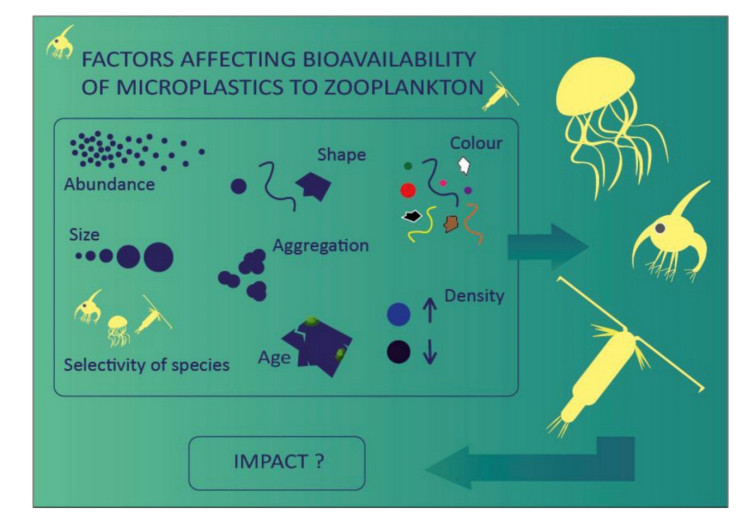
Botterell Z, Beaumont N, Dorrington T, et al. (2019) Bioavailability and effects of microplastics on marine zooplankton: A review. Environ Poll 245: 98–110. doi: 10.1016/j.envpol.2018.10.065
    [30] de Orte MS, Clowez S, Caldeira K (2019) Response of bleached and symbiotic sea anemones to plastic microfiber exposure. Environ Poll 249: 512–517. doi: 10.1016/j.envpol.2019.02.100
    [31] Cole M, Lindeque P, Fileman E, et al. (2013) Microplastic ingestion by zooplankton. Envir Sci Tech 47: 6646–6655. doi: 10.1021/es400663f
    [32] Mohsen M, Wang Q, Zhang L, et al. (2019) Microplastic ingestion by the farmed sea cucoumber Apostichopus japonicus in China. Environ Pollut 245: 1071–1078. doi: 10.1016/j.envpol.2018.11.083
    [33] Grigorakus S, Mason S, Drouillard K (2017) Determination of the gut retention of plastic microbeads and microfibers in goldfish (Carassius auratus). Chemosphere 169: 233–238. doi: 10.1016/j.chemosphere.2016.11.055
    [34] Besseling E, Wegner A, Foekema EM, et al. (2013) Effects of microplastics on fitness and PCB bioaccumulation by the lugworm Arenicola marina (L.). Environ Sci Tech 47: 593–600. doi: 10.1021/es302763x
    [35] Setälä O, Fleming-Lehtinen V, Lehtiniemi M (2014) Ingestion and transfer of microplastics in the planktonic food web. Environ Poll 185: 77–83. doi: 10.1016/j.envpol.2013.10.013
    [36] Woods M, Stack M, Fields D, et al. (2018) Microplastic fiber uptake, ingestion, and egestion rates in blue mussel (Mytilus edulis). Mar Poll Bull 137: 638–645. doi: 10.1016/j.marpolbul.2018.10.061
    [37] Li L, Cai H, Rochman C, et al. (2019) The uptake of microfibers by freshwater Asian clams (Corbicula fluminea) varies based upon physicochemical properties. Chemosphere 221: 107–114. doi: 10.1016/j.chemosphere.2019.01.024
    [38] Watts AJ, Urbina MA, Goodhead R, et al. (2016) Effect of microplastic on the gills of the shore crab Carcinus maenas. Environ Sci Technol 50: 5364–5369. doi: 10.1021/acs.est.6b01187
    [39] Lu Y, Zhang Y, Deng Y, et al. (2016) Uptake and accumulation of polystyrene microplastics in zebrafish (Danio rerio) and toxic effects in liver. Envir Sci Tech 50: 4054–4060. doi: 10.1021/acs.est.6b00183
    [40] Collard F, Gilbert B, Compere P, et al. (2017) Microplastics in the livers of European anchovies (Engraulis encrasicolus L.). Environ Poll 229: 1000–1005. doi: 10.1016/j.envpol.2017.07.089
    [41] Rosenkrantz P, Chaudhry Q, Stone V, et al. (2009) A comparison of nanoparticle and fine particle uptake by Daphnia magna. Environ Toxicol Chem 28: 2142–2149. doi: 10.1897/08-559.1
    [42] Schür C, Rist S, Baun A, et al. (2019) When fluorescence is not a particle: The tissue translocation of microplastics in Daphnia magna seems an artifact. Environ Toxicol Chem
    [43] Farrell P, Nelson K (2013) Trophic level transfer of microplastic: Mytilus edulis (L.) to Carcinus maenas (L.). Envir Poll 177: 1–3.
    [44] Santana M, Moreira F, Turra A (2017) Trophic transference of microplastics under a low exposure scenario: insights on the likelihood of particle cascading along marine food webs. Mar Poll Bull 121: 154–159. doi: 10.1016/j.marpolbul.2017.05.061
    [45] Haegerbaeumer A, Mueller MT, Fueser H, et al. (2019) Impacts of micro-and nano-sized plastic particles on benthic invertebrates: A literature review and gap analysis. Front Envir Sci 7: 17. doi: 10.3389/fenvs.2019.00017
    [46] Rillig M, Ziersch L, Hempel S (2017) Microplastic transport in soil by earthworms. Sci Reports 7. Article number 1362.
    [47] Zhu F, Zhu C, Wang C, et al. (2019) Occurrence and ecological impacts of microplastics in soil systems: A review. Bull Environ Contam Toxicol 102: 741–749. doi: 10.1007/s00128-019-02623-z
    [48] Prendergast-Miller M, Katsiamides A, Abbass, M, et al. (2019) Polyester-derived microfibre impacts on the soil dwelling earthworm, Lumbricus terrestris. Environ Pollut 251: 453–459. doi: 10.1016/j.envpol.2019.05.037
    [49] Lwanga E, Gertsen H, Gooren H (2016) Microplastics in the terrestrial ecosystem: Implications for Lumbricus terrestris (Oligochaeta, Lumbricidae). Environ Sci Tech 505: 2685–2691.
    [50] Green D, Colgan T, Thompson R, et al. (2019) Exposure to microplastics reduces attainment strength and alters the haemolymph proteome of blue mussels (Mytilus edulis). Envir Poll 246: 423–434. doi: 10.1016/j.envpol.2018.12.017
    [51] Au S, Bruce T, Bridges W (2015) Responses of Hyalella azteca to acute and chronic microplastic exposures. Environ Toxicol Chem 34: 2564–2572. doi: 10.1002/etc.3093
    [52] Jovanovic B (2017) Ingestion of microplastic by fish and its potential consequences from a physical perspective. Integr Environ Assess Managmt 13: 510–515. doi: 10.1002/ieam.1913
    [53] Bour A, Haarr A, Keiter S, et al. (2018) Environmentally relevant microplastic exposure affects sediment-dwelling bivalves. Envir Poll 236: 652–660. doi: 10.1016/j.envpol.2018.02.006
    [54] Ziajahromi S, Kumar A, Neale P, et al. (2017) Impact of microplastic beads and fibers on waterflea (Ceriodaphnia dubia) survival, growth, and reproduction: Implications of single and mixture exposures. Environ Sci Technol 51: 13397–13406. doi: 10.1021/acs.est.7b03574
    [55] Foley CJ, Feiner ZS, Malinich TD, et al. (2018) A meta-analysis of the effects of exposure to microplastics on fish and aquatic invertebrates. Sci Total Envir 631–632: 550–559.
    [56] Rochman C, Hoh E, Hentschel B, et al. (2013) Long-term field measurement of sorption of organic contaminants to five types of plastic pellets: implications for plastic marine debris. Environ Sci Tech 47: 1646–1654.
    [57] Rochman C, Hoh E, Kurobe T, et al. (2013) Ingested plastic transfers hazardous chemicals to fish and induces hepatic stress. Sci Rep 3: 3263. doi: 10.1038/srep03263
    [58] Rochman C, Hentschel B, Teh S (2014) Long-term sorption of metals is similar among plastic types: implications for plastic debris in aquatic environments. PloS One 9: e85433. doi: 10.1371/journal.pone.0085433
    [59] Seuront L (2018) Microplastic leachates impair behavioural vigilance and predator avoidance in a temperate intertidal gastropod. Biol Lett 14: 20180453. doi: 10.1098/rsbl.2018.0453
    [60] Pannetier P, Morin B, Clérandeau C, et al. (2019) Toxicity assessment of pollutants sorbed on environmental microplastics collected on beaches: Part II – adverse effects on Japanese medaka early life stages. Environ Poll 248: 1098–1107. doi: 10.1016/j.envpol.2018.10.129
    [61] Wardrop P, Shimeta J, Nugegoda D, et al. (2016) Chemical pollutants sorbed to ingested microbeads from personal care products accumulate in fish. Environ Sci Technol 50: 4037–4044. doi: 10.1021/acs.est.5b06280
    [62] Beckingham B, Ghosh U (2017) Differential bioavailability of polychlorinated biphenyls associated with environmental particles: Microplastic in comparison to wood, coal and biochar. Environ Poll 220: 150–158. doi: 10.1016/j.envpol.2016.09.033
    [63] Hodson M, Duffus-Hodson C, Clark A (2017) Plastic bag derived microplastics as a vector for metal exposure in terrestrial invertebrates. Environ Sci Tech 518: 4714–4721.
    [64] Tourinho P, Koci V, Loureiro S, et al. (2019) Partitioning of chemical contaminants to microplastics: Sorption mechanisms, environmental distribution and effects on toxicity and bioaccumulation. Envir Pollut 252: 1246–1256. doi: 10.1016/j.envpol.2019.06.030
    [65] Batel A, Linti F, Scherer M, et al. (2016) Transfer of benzo [a] pyrene from microplastics to Artemia nauplii and further to zebrafish via a trophic food web experiment: CYP1A induction and visual tracking of persistent organic pollutants. Environ Toxicol Chem 35: 1656–1666. doi: 10.1002/etc.3361
    [66] Bakir A, Rowland S, Thompson R (2014) Enhanced desorption of persistent organic pollutants from microplastics under simulated physiological conditions. Environ Poll 185: 16–23. doi: 10.1016/j.envpol.2013.10.007
    [67] Bakir A, O'Connor I, Rowland S, et al. (2016) Relative importance of microplastics as a pathway for the transfer of hydrophobic organic chemicals to marine life. Environ Poll 219: 56–65. doi: 10.1016/j.envpol.2016.09.046
    [68] Ziajahromi S, Kumar A, Neale P (2019) Effects of polyethylene microplastics on the acute toxicity of a synthetic pyrethroid to midge larvae (Chironomus tepperi) in synthetic and river water. Sci Total Envir 671: 971–975. doi: 10.1016/j.scitotenv.2019.03.425
    [69] Wang J, Coffin S, Sun C, et al. (2019) Negligible effects of microplastics on animal fitness and HOC bioaccumulation in earthworm Eisenia fetida in soil. Environ Pollut 249: 776–784. doi: 10.1016/j.envpol.2019.03.102
    [70] McIlwraitha H, Lina J, Erdleb L, et al. (2019) Capturing microfibers – marketed technologies reduce microfiber emissions from washing machines. Mar Poll Bull 139: 40–45. doi: 10.1016/j.marpolbul.2018.12.012
    [71] Weis JS (2018) Cooperative work is needed between textile scientists and environmental scientists to tackle the problems of pollution by microfibers. J Textile Apparel Tech Mgmt 10: 1–3.
    [72] Almroth B, Åström L, Roslund S, et al. (2018) Quantifying shedding of synthetic fibers from textiles; a source of microplastics released into the environment. Envi Sci Poll Res 25: 1191–1199. doi: 10.1007/s11356-017-0528-7
    [73] Zambrano M, Pawlak J, Daystar J, et al. (2019) Microfibers generated from the laundering of cotton, nylon, and polyester based fabrics and their aquatic degradation. Mar Poll Bull 142: 394–407. doi: 10.1016/j.marpolbul.2019.02.062
    [74] Belzagui F, Crespi M, Álvarez A, et al. (2019) Microplastics' emission: microfibers' detachment from textile garments. Envir Poll 248: 1028–1035. doi: 10.1016/j.envpol.2019.02.059
    [75] Pena-Francesch A, Demirel M (2019) Squid-inspired tandem repeat proteins: Functional fibers and films. Front Chem 7: 69. doi: 10.3389/fchem.2019.00069
  • This article has been cited by:

    1. P. M.A. Sloot, S. V. Ivanov, A. V. Boukhanovsky, D. A.M.C. van de Vijver, C. A.B. Boucher, Stochastic simulation of HIV population dynamics through complex network modelling, 2008, 85, 0020-7160, 1175, 10.1080/00207160701750583
    2. Arni S.R. Srinivasa Rao, A note on derivation of the generating function for the right truncated Rayleigh distribution, 2006, 19, 08939659, 789, 10.1016/j.aml.2005.04.018
    3. Angelina Mageni Lutambi, The effect of delayed death in HIV/AIDS models, 2016, 10, 1751-3758, 286, 10.1080/17513758.2016.1179801
    4. Arni S.R. Srinivasa Rao, Incubation periods under various anti-retroviral therapies in homogeneous mixing and age-structured dynamical models: A theoretical approach, 2015, 45, 0035-7596, 10.1216/RMJ-2015-45-3-973
  • Reader Comments
  • © 2019 the Author(s), licensee AIMS Press. This is an open access article distributed under the terms of the Creative Commons Attribution License (http://creativecommons.org/licenses/by/4.0)
通讯作者: 陈斌, bchen63@163.com
  • 1. 

    沈阳化工大学材料科学与工程学院 沈阳 110142

  1. 本站搜索
  2. 百度学术搜索
  3. 万方数据库搜索
  4. CNKI搜索

Metrics

Article views(7841) PDF downloads(1882) Cited by(26)

Figures and Tables

Figures(1)

Other Articles By Authors

/

DownLoad:  Full-Size Img  PowerPoint
Return
Return

Catalog