A conservation law with multiply discontinuous flux modelling a flotation column

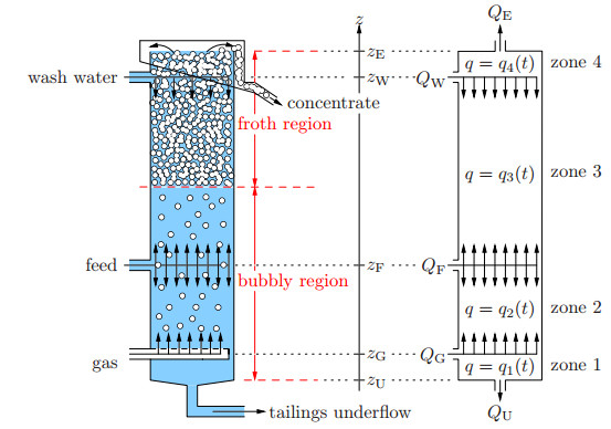
1.   Introduction

A turbidostat, similar to a chemostat or an auxostat, is a basic piece of laboratory apparatus used to cultivate microorganisms, and it has feedback between the concentration of the fluid in the culture dish and the dilution rate ^[1,2,3,4,5]. Compared with the chemostat ^[6,7], the turbidostat can feed back the state values to the controller through the photoelectric system to control the flow rate of the limiting nutrient in the fresh inflowing medium according to the concentration of the fluid in the culture dish, so as to achieve the purpose of high-efficiency culture. The device used to measure the concentration of the liquid is called the optical sensor, which can measure both the microbial species concentration and the substrate concentration ^[8,9]. At present, there are a variety of microorganisms that can be continuously fermented by large-size turbidostats according to this principle in the fermentation industry. Microbial metabolites in balance with the bacteria can also be produced by continuous fermentation with a turbidostat. In consideration of the important value of the turbidostat in theory and practical application, the research on the kinetic model of the turbidostat has attracted the attention of many biologists, experimental technicians and mathematicians ^{[10,11,12,13,14,15,16]}. Leenheer and Smith ^[10] investigated the coexistence of two species in a turbidostat model with monotonic uptake functions by dint of feedback control of the dilution rate. In ^[11], a turbidostat model of exploitative competition for an inhibitory growth-limiting nutrient between two species of microorganisms was considered. Further, the author of ^[12] analyzed the dynamics of a turbidostat model with a non-monotonic response function and found that the coexistence can be dependent on the original condition if the washout equilibrium and the interior equilibrium are asymptotically stable synchronously.

However, in reality, no matter how sensitive a piece of online equipment used to measure nutrient or microorganism concentrations is, there invariably exists a time delay in the measurement of the concentration of the fluid and when this signal can be available to regulate the input flow rate. That is, online equipment typically only provides delayed discrete measurements. In ^[17], Mikheev et al. considered a digital controlled continuous-time system as a continuous-time system with time-varying delayed control input, and then Fridman ^[18] further researched the control system which can be described in the form of differential equations with after-effects. Subsequently, turbidostat systems with delayed feedback control have been investigated by multitudinous researchers ^{[19,20,21,22,23,24,25]}. Yuan et al. ^[22] revealed that the time delay may lead to the loss of stability and generate various oscillations and periodic solutions under the condition that the dilution rate depends on the turbidity of two competing species. In ^[19], by taking the dilution rate related to the substrate concentration as a feedback control variable, the author studied the asymptotic stabilization for a turbidostat by considering a delay on its output. A feedback analysis for turbidostats whose growth functions can be nonmonotonic was carried out in ^[23], where the dilution rate rests with the substrate concentration with piecewise constant delayed measurements.

Inevitably, population dynamics are susceptible to environmental noise in almost all ecological systems, which primarily involves continuous white noise. Under well-controlled laboratory conditions, even if the observed experimental results are very consistent with the theoretical behaviors of ordinary differential equations in the turbidostat system, the possible differences under operational conditions cannot be neglected. By introducing white noise, the dynamics of turbidostat models can be better understood ^{[26,27,28,29,30,31]}. The persistence in mean and stochastic persistence of a stochastic turbidostat model were obtained ^[32], as white noise is introduced by the maximal growth rate. Mu et al. ^[33] obtained sufficient conditions for competitive exclusion among microorganisms. In ^[34], Li et al. derived conditions of mean persistence and extinction for the population and showed that the species may survive when the disturbance is small enough.

Some researchers have taken into account both delay and stochastic phenomena in turbidostat for microbial culture ^[35,36]. However, for all we know, there are few works of literature considering the stochastic turbidostat model with piecewise constant delayed feedback control. In our work, we delve into the dynamical behaviors of the species in the turbidostat with both piecewise constant delayed feedback control and environmental random fluctuation. The rest of this paper is furnished as follows: In Section 2, we put forward the stochastic turbidostat model with a controllable dilution rate, where feedback depends on piecewise constant delayed measurements of the substrate level. The existence and uniqueness of the global positive solution of the model are presented in Section 3. We probe into the extinction and persistence of the species separately in Section 4. Section 5 deals with the stochastic asymptotical stability of the washout equilibrium and the asymptotic behavior of the stochastic delayed model around the interior equilibrium of the corresponding deterministic delayed model. Section 6 offers some numerical examples. The meanings of our results are briefly discussed in the final section.

2.   The model

Gonzalo ^[19] considered a turbidostat model with discrete delay $ \tau > 0 $ on the output:

where $ S(t) $ and $ x(t) $ depict the substance and the microbial species levels at time $ t, $ respectively. $ s_{in} > 0 $ represents the input concentration of the substrate. $ \tau $ is the delay of the optical sensor in the measurement of the concentration of the fluid. In the turbidostat, the concentration of the limiting nutrient in the container possesses a feedback control effect on the input rate of the fresh nutrient. Therefore, the input flow rate $ D(S(t-\tau)) > 0 $ can be manipulated and depends on the substrate level at time $ t-\tau $. The function $ \mu:\mathbb{R}_+ \mapsto \mathbb{R}_+ $ stands for the uptake rate at which nutrient is absorbed by the species and is assumed to be a continuously differentiable function.

The measurements of the concentration of the fluid in ^[19] are assumed to be continuous. However, given that the sample data provided by online devices are discrete, we consider the following piecewise-linear delay. Fix any two positive numbers $ \varepsilon_1, \varepsilon_2 > \varepsilon_1 $ such that a sequence of real numbers $ \{t_i\} $ satisfies $ 0 < \varepsilon_1\leq t_{i+1}-t_i\leq \varepsilon_2 $ for every $ i\in \mathbb{N} \cup \{0\} $, where $ t_0 = 0 $ and $ \mathbb{N} = \{1, 2, \ldots\} $. Given an arbitrary constant $ \tau_f \geq0 $, we give the following function $ \tau(t) $:

Employing the above definition, it follows that $ t-\tau(t) = t-(\tau_{f}+t-t_j) = t_j-\tau_{f} $ for every $ j\geq0 $ and $ t\in [t_j+\tau_{f}, t_{j+1}+\tau_{f}) $, which means $ t-\tau(t) $ is piecewise constant. In the particular case of $ \tau_f = 0 $, $ t-\tau(t) = t_j $ for any $ t\in [t_j, t_{j+1}), j\geq0 $. In addition, for every $ t\geq0 $, one obtains $ 0\leq\tau(t)\leq\tau_{M} $, where $ \tau_{M} = 2\tau_{f}+\varepsilon_2 $. In this case, the measurement available $ S(t-\tau) $ in model (2.1) can be rewritten as $ S(t-\tau(t)) $.

Microorganisms consume nutrients for growth, which leads to a decrease in nutrients in the turbidostat. We adopt the function of the form

to describe the consumption, where $ m $ is the maximal uptake rate. The derivative of $ f(S(t)) $ satisfies $ f'(S(t)) > 0 $, and $ f_1(S(t)) $ is a bounded continuous function on any finite interval. The presence of ambient noise makes the arguments contained in model (2.1) always swing near some average values rather than reaching fixed values over the time evolution. As one of the pivotal arguments in the turbidostat model, the maximum uptake rate of the organism is more susceptible to environmental noise ^{[26,27,31,32]}. Under the circumstances, randomness can be introduced into the maximal uptake rate $ m $ such that $ m\rightarrow m+ \sigma B(t) $, where the $ B(t)\in(\Omega, \mathscr{F}, \mathscr{F}_{t\geq0}, \mathcal{P}) $ applied to imitate the stochastic effect is standard Brownian motion, and $ \sigma $ reflects the intensity of the white noise. In consequence, we use $ m + \sigma B (t) $ instead of $ m $ in the deterministic model (2.1) to obtain the following stochastic differential equation model with piecewise constant delayed measurements of the substrate level:

with initial value conditions

The only control variable, the dilution rate $ D(S(t-\tau(t))) $, can be defined by $ D(S(t-\tau(t))) = h(S^*-S(t-\tau(t))) $ so that the nutrient concentration can approach $ S^{*} $ with an appropriate feedback control law, where $ S^{*} $ is the desired substrate level. Suppose that the function $ h $ fulfills the following conditions:

$ {\bf{(A1)}} $ The continuous differentiable function $ h:\mathbb{R} \mapsto \mathbb{R}_+ $ is positive, bounded, increasing and satisfies $ mf(S^*) = h(0) $.

$ {\bf{(A2) }}$ There is a unique root $ S^*\in(0, s_{in}) $ such that the equation $ mf(S)-h(S^*-S) = 0 $ holds.

Quite evidently, this type of feedback control is set up so that the corresponding deterministic delayed model of model (2.2) possesses a washout equilibrium $ E_0 = (s_{in}, 0) $ and a unique positive equilibrium $ E^* = (S^*, x^*) $, where $ x^* = s_{in}-S^* $. The positive equilibrium point can be set in advance, which means that we can control and achieve our expectations by imposing some conditions. Hence, the control problem we consider is to find sufficient conditions for the persistence of the species, even to make the concentration of the species close to $ s_{in}-S^* $ under the influence of delayed measurements and random perturbation. These questions are to be answered next.

3.   Existence and uniqueness of the positive solution

In consideration of ecological and mathematical significance, whether there exists a global unique positive solution is our primary concern. For this purpose, it is generally required that the arguments of (2.2) fulfill the local Lipschitz condition and the linear growth condition ^[37]. Whereas the parameters of model (2.2) do not satisfy the linear growth condition, the solutions may explode in a limited time. In this section, we analyze the existence of the unique global positive solution of model (2.2).

Theorem 3.1. For any initial value (2.3), model (2.2) admits a unique global solution $ (S(t), x(t)) $ on $ t\geq-\tau_M, $ and the solution will remain in $ \mathbb{R}_{+}^2 $ with probability one; that is, $ (S(t), x(t))\in \mathbb{R}_{+}^2 $ for all $ t\geq-\tau_M $ almost surely $ (a.s.) $.

Proof. In the light of approaches in ^[37], model (2.2) possesses a unique local positive solution $ (S(t), x(t)) $ on $ t\in[-\tau_M, \varsigma_{e}) $, where $ \varsigma_{e} $ is the blow up time, which means the trajectories may diverge to infinity as $ t $ goes to the finite time $ \varsigma_e $. In order to get globality of the solution, we only need to demonstrate $ \varsigma_e = \infty $ a.s.

Let $ z(t) = s_{in}-S(t)-x(t) $. Then,

whose solution is expressed as

which results in $ S(t)+x(t)\leq \max\{\varphi_{1}(0)+\varphi_{2}(0), 2s_{in}-\varphi_{1}(0)-\varphi_{2}(0)\} = M $ for all $ t < \varsigma_{0} $, where

It is clear that $ \varsigma_{0}\leq\varsigma_{e} $ a.s. In order to get $ \varsigma_{e} = \infty $, we only need to show that $ \varsigma_{0} = \infty $ a.s. Now, we select $ \epsilon_{0} > 0 $ such that $ \varphi_{1} (\vartheta) > \epsilon_{0}, \varphi_{2}(\vartheta) > \epsilon_{0}. $ For $ 0 < \epsilon\leq\epsilon_{0}, $ define the following stopping time:

The empty set is generally denoted as $ \varnothing $. Let $ \inf\varnothing = \infty $ all through this paper. There is no doubt that $ \varsigma_{\epsilon} $ is increasing as $ \epsilon $ approaches 0. Therefore, $ \varsigma_{0} = \lim_{\epsilon\rightarrow0}\varsigma_{\epsilon} $ a.s. Next, the proof can be accomplished if we get $ \varsigma_{0} = \infty $ a.s.

For proof by contradiction, assume that there exists a pair of positive numbers $ \delta\in(0, 1) $ and $ T\in[t_{i}, t_{i+1}) $ such that $ \mathbb{P}\{\varsigma_{0}\leq T\} > \delta $, where $ i\in \mathbb{N} \cup \{0\} $. Thus, there is a constant $ \epsilon_{1}\in(0, \epsilon_{0}) $ such that $ \mathbb{P}\{\varsigma_{\epsilon}\leq T\} > \delta $ for any $ 0 < \epsilon\leq\epsilon_{1} $.

Additionally, define a $ \mathbb{C}^{2} $-function $ V: \mathbb{R}_{+}^{2}\to \mathbb{R}_{+} $ by

Obviously, $ V(S, x) $ is positive definite for all $ S, x > 0. $ Using Itô's formula to model (2.2), one derives

where

where $ \tilde{M} $ is the upper bound of the function $ f_1(S) $ on $ [0, M] $. Accordingly, we obtain

Integrating and taking the expectation of both sides of (3.3) yield

and

Superimposing the above inequations, we can get

For any $ 0 < \epsilon\leq\epsilon_{1} $, we set $ \Omega_{\epsilon} = \{\varsigma_{\epsilon}\leq T\} $, and then $ \mathbb{P}(\Omega_{\epsilon}) > \delta. $ On the grounds of the definition of the blow up time, there exists $ S\left({{\varsigma }_{\epsilon}}, \omega \right) $, or $ x\left({{\varsigma }_{\epsilon}}, \omega \right) $ equals $ \epsilon $ for every $ \omega \in {{\Omega }_{\epsilon}} $, and then

Via (3.4), one infers

This leads to a contradiction as we let $ \epsilon\to 0 $,

So, we get $ {{\varsigma }_{0}} = \infty $ a.s. The proof is completed.

Define

It suffices from (3.2) to display that $ \Lambda $ is the positive invariant set of model (2.2). Throughout this paper, we always assume that the starting value $ (\varphi_1, \varphi_2) $ is constrained in $ \Lambda $.

4.   Extinction and permanence

This section provides sufficient conditions for strong stochastic persistence and extinction of the microorganism in the turbidostat. For the sake of convenience, denote

Then, we define

and

4.1.   Extinction

The following theorem is about the extinction of the microorganism.

Theorem 4.1. The biomass $ x(t) $ will die out exponentially, namely, $ \lim_{t\rightarrow \infty}x(t) = 0 $ a.s., provided

$ {\bf{(i)}} $ $ h(S^*-s_{in}) < mf(s_{in})\leq 2h(S^*-s_{in}) $ and $ \lambda_1 < 0 \ (i.e. \ \sigma > \frac{\sqrt{2(mf(s_{in})-h(S^*-s_{in}))}}{f(s_{in})}) $; or

$ {\bf{(ii) }}$ $ mf(s_{in}) > 2h(S^*-s_{in}) $ and $ \sigma > \frac{m}{\sqrt{2h(S^*-s_{in})}} $.

Proof. In order to discuss the extinction of the biomass, applying It$ \hat{o} $'s formula to $ W_1(x) = \ln x $ yields

By integrating on the both sides of the above inequality from 0 to $ t $, we can obtain

which further results in

where $ \overline{W}_1 $ is an upper bound of the function $ LW_1 = f(S)\left(m-\frac{1}{2}\sigma^{2}f(S)\right)-h(S^{*}-s_{in}) $, and $ \psi(t) = \frac{1}{t}\left[\ln x(0)+\int_{0}^{t}\sigma f(S(r))\mathrm{d}B(r)\right]. $ According to the strong law of large numbers for local martingale, we get $ \lim_{t\rightarrow \infty}\psi(t) = 0 $ a.s., which means $ \limsup_{t\rightarrow \infty}\frac{\ln x(t)}{t}\leq\overline{W}_1 $ a.s. To get the extinction of $ x(t) $, we need to show $ \overline{W}_1 < 0 $.

Next, we consider two cases by treating the function $ f(S)\left(m-\frac{1}{2}\sigma^{2}f(S)\right) $ as a quadratic function about $ f(S) $. Case (i): On the premise of $ h(S^*-s_{in}) < mf(s_{in})\leq 2h(S^*-s_{in}) $, when $ \sigma^2\leq\frac{m}{f(s_{in})} $, the function $ f(S)\left(m-\frac{1}{2}\sigma^{2}f(S)\right) $ is increasing for $ S\in[0, s_{in}] $. Then, we have $ LW_1\leq mf(s_{in})-h(S^{*}-s_{in})-\frac{1}{2}\sigma^{2}f^{2}(s_{in}) = \lambda_1 < 0 $, which means $ \overline{W}_1 < 0 $ if $ mf(s_{in})-h(S^*-s_{in}) < \sigma^2\leq\frac{m}{f(s_{in})} $. For $ \sigma^2 > \frac{m}{f(s_{in})} $, the function $ f(S)\left(m-\frac{1}{2}\sigma^{2}f(S)\right) $ reaches the maximum value when $ f(S) = \frac{m}{\sigma^2} $, and then we have $ LW_1\leq \frac{m^2}{2\sigma^2}-h(S^{*}-s_{in}) < \frac{mf(s_{in})}{2}-h(S^{*}-s_{in}) < 0 $. To sum up, if $ h(S^*-s_{in}) < mf(s_{in})\leq 2h(S^*-s_{in}) $ and $ \lambda_1 < 0 $, the biomass $ x(t) $ will die out. Case (ii): In the case of $ mf(s_{in}) > 2h(S^*-s_{in}) $, one obtains $ LW_1\leq mf(s_{in})-h(S^{*}-s_{in})-\frac{1}{2}\sigma^{2}f^{2}(s_{in}) $ when $ \sigma^2\leq\frac{m}{f(s_{in})} $; nevertheless, at this point $ mf(s_{in})-h(S^{*}-s_{in})-\frac{1}{2}\sigma^{2}f^{2}(s_{in}) > 0 $. On the contrary, when $ \sigma^2 > \frac{m}{f(s_{in})} $, we have $ LW_1\leq \frac{m^2}{2\sigma^2}-h(S^{*}-s_{in}) < 0 $ owing to $ \sigma > \frac{m}{\sqrt{2h(S^*-s_{in})}} > \sqrt{\frac{m}{f(s_{in})}} $. Hence, if $ mf(s_{in}) > 2h(S^*-s_{in}) $ and $ \sigma > \frac{m}{\sqrt{2h(S^*-s_{in})}} $, the microorganism $ x(t) $ will be extinct. The proof is completed.

In line with Theorem 4.1, it can be validated that stochasticity will result in the disappearance of the species of model (2.2) when the magnitude of stochasticity is large enough. In contrast, how does the biomass change in the turbidostat in the case of small intensity of disturbance? In the following, we discuss the stochastic strong permanence of the microorganism.

4.2.   Stochastic strong permanence

This subsection is intended for stochastic strong permanence of the biomass of model (2.2) under the influence of small noise. To figure out the permanence of the microorganism for model (2.2), we introduce the equation

with initial value $ \varphi_2 $. Let us first prepare the following useful lemma.

Lemma 4.1. Denote $ \partial\Lambda: = \{(S, x)\in\Lambda:x = 0\} $. Then, there is a $ T > 0 $ such that

for any $ (\varphi_1, \varphi_2)\in\partial\Lambda $, where $ \tilde{F}(S(t)) = -\frac{1}{2}\sigma^2f^2(S)+mf(S)-h(S^*) $.

Proof. If $ \varphi_2 = 0, $ then $ x(t) = 0 $ for all $ t \geq-\tau_M $, and the first equation of model (2.2) turns into

Apparently, the solution of (4.3) converges to $ s_{in} $. Consequently,

for every $ (\varphi_1, \varphi_2)\in\partial\Lambda $. Then, we can find a positive number $ T $ fulfilling (4.2).

Theorem 4.2. If $ \lambda_2 > 0, $ then $ X(t) $ of model (4.1) is strongly stochastically permanent, that is, for any $ \gamma > 0 $, there exists a $ \alpha_1 > 0 $ such that

Proof. Introduce a Lyapunov function $ W_\theta = X^\theta $, where $ \theta\in \mathbb{R} $ is a constant that needs to be specified. Simple calculations for $ W_\theta $ on the grounds of It$ \hat{o} $'s formula give

Define $ \mathcal{O_\theta} = \sup_{(S, X)\in \Lambda}\left\{\theta\left[mf(S)-h(S^*)+\frac{\theta-1}{2}\sigma^2f^2(S)\right]\right\} $. Then, for any starting value $ \varphi_2 $, we get from (4.4) that $ LW_\theta\leq\mathcal{O_\theta}X^\theta $. By applying It$ \hat{o} $'s formula and taking expectations, we obtain

for any $ t\geq0 $, $ \varphi_2 > 0 $. On the basis of It$ \hat{o} $'s formula, (4.1) becomes

Integrating both sides of the above equality from 0 to $ t $ yields

Define $ W_2(t) = \ln X(0)-\ln X(t) $. From (4.6), one has

According to Lemma 4.1 and Feller property, it then follows from the above equation that we can find a sufficiently small $ \delta_1 > 0 $ such that

for $ \varphi_2 < \delta_1 $. In the light of (4.5), for any fixed $ t\geq0 $, we get

It then suffices from [38, Lemma 2.2] to show that

where $ \mathcal{\tilde{O}} $ is a constant which is dependent on $ T $, $ \mathcal{O}_{-1} $ and $ \mathcal{O}_1 $. If $ \theta $ is sufficiently small and fulfills $ \mathcal{\tilde{O}}\theta^2\leq\frac{\lambda_2\theta T}{4} $, we get from (4.7) that

which further implies

for $ \varphi_2 < \delta_1 $, where $ c_1 = \exp(-\frac{\lambda_2\theta T}{4}) $. Noting (4.5), we obtain

for any $ \varphi_2 > \delta_1 $. This, combined with (4.8), means that

for any $ \varphi_2 $. Considering that the Markov property, the following inequation

holds for any $ \varphi_2 $. By the method of recursion, we obtain

This together with (4.5) results in

Consequently,

as $ n\rightarrow \infty $. The theorem easily follows from an application of Markov's inequality to the above inequation.

Combining Theorem 4.2 and the comparison principle, we conclude the following theorem about the permanence of the microorganism $ x(t) $ of model (2.2).

Theorem 4.3. The microorganism $ x(t) $ is strongly stochastically permanent provided $ \lambda_2 > 0 $.

In the contents above, the microorganism may die out in the case that the magnitude of stochasticity is sufficiently large, and the microorganism will be strongly stochastically permanent when the magnitude is small enough. Nevertheless, what we're more curious about is whether the microorganism fluctuates near the wanted biomass concentration $ s_{in}-S^* $ under the combined action of delayed measurements and random disturbance. Therefore, in the rest of this article, we will make an investigation on the asymptotic behaviors of model (2.2) around the steady states of the corresponding deterministic delayed model.

5.   Analysis of asymptotic behaviors

In this section, we look into the asymptotic stability of the washout equilibrium and asymptotic behavior of model (2.2) around the interior equilibrium $ E^* $ of its corresponding deterministic delayed model.

Theorem 5.1. Assume that $ \lambda_1 < 0 $; then, the washout equilibrium $ E_0 = (s_{in}, 0) $ is asymptotically stable in probability.

Proof. Set the Lyapunov function

where $ p\in (0, 1) $ will be determined later. Applying It$ \hat{o} $'s formula to (5.1) yields

Noticing that $ \lambda_1 < 0 $, we can choose sufficiently small positive numbers $ p, \nu $ such that $ -2h(S^{*}-S(t-\tau(t)))\leq-2h(S^{*}-s_{in})\leq p(\lambda_1+\nu) < 0 $. Let $ D_{\delta_{1}}: = (s_{in}-\delta_{1}, s_{in}]\times[0, \delta_{1}) $ for $ \delta_{1}\in (0, s_{in}) $. For any $ (S, x)\in D_{\delta_{1}} $, $ x $ has a tendency to 0 as $ \delta_1 $ approaches to $ 0^+ $, which combined with the continuity of $ F(S, x) $ leads to

If $ p $ and $ \delta_1 $ are small enough, the following inequation holds:

for any $ (S, x)\in D_{\delta_{1}} $, where $ 0 < \nu_1, \nu_2 < \nu $ and $ \nu = \nu_1+\nu_2 $. Hence, for any $ (S, x)\in D_{\delta_{1}} $, we obtain

By virtue of [38, Theorem 3.1], we deduce that the microorganism-free equilibrium $ (s_{in}, 0) $ is asymptotically stable in probability.

Our control target is to make the random paths close to $ E^{*} $ with a delayed state feedback of the form $ h(S^{*}-S(t-\tau(t))). $ Whereas, $ E^{*} $ is no longer the equilibrium of stochastic delayed model (2.2), the asymptotic behavior of model (2.2) around the steady state $ E^{*} $ will be discussed.

For convenience of the analysis below, we introduce some notations:

Theorem 5.2. Suppose that $ \lambda_2 > 0 $ and

Then, there exists $ T_2 > 2\tau_M $ such that

where

Proof. Noting that $ \lambda_2 > 0 $, by Theorem 4.3, we can choose a pair of positive numbers $ T_{1} $ and $ \alpha_2 < \min\{s_{in}-S^*, \alpha_1\} $ satisfying $ x(t)\geq\alpha_2 $ a.s. for all $ t\geq T_{1} $. Thus,

It follows that $ S_{a}\in(S^*, s_{in}) $ owing to $ 0 < \alpha_{2} < s_{in}-S^* < s_{in} $ for $ t\geq T_{1}. $ On account of the mean value theorem, we can get that

where $ \xi\in[0, S^{*}-S(t-\tau(t))] $ or $ [S^{*}-S(t-\tau(t)), 0]. $ By the inequality $ 2ab\leq a^{2}+b^{2}, $ we infer

for all $ t\geq T_{1}+2\tau_M $.

We define a Lyapunov functional $ U_{1} $ as follows:

which is nonnegative and belongs to class $ \mathbb{C}^{1} $ over $ [0, s_{in}) $. It follows from (5.3) that its derivative along all trajectories of model (2.2) for any $ t\geq T_{1}+2\tau_M $ satisfies

where $ \eta\in[S^{*}, S(t)] $ or $ [S(t), S^{*}]. $

Construct a differentiable function $ U_{2}, $ whose specific mathematical expression is

A preliminary calculation gives, for any $ t\geq T_{1}+2\tau_M, $

Taking the integral from $ T_{2} > T_{1}+2\tau_M $ to $ t $ and then taking the expectation, we have

On the basis of the Burkholder-Davis-Gundy inequality, we get

It suffices from Fubini's Theorem to obtain

Hence,

Taking the superior limit of both sides of (5.5) leads to

This completes the proof of Theorem 5.2.

Remark 5.1. In view of Theorem 5.2, when the magnitude of stochasticity and the delay of measurements are small, the expected time average of the distance between the equilibrium $ E^* $ and the stochastic solution $ (S(t), x(t)) $ will finally bind in a narrow area. That is, the solutions of stochastic delayed model (2.2) will be swinging around a point near the steady state $ E^{*} $ of the corresponding deterministic delayed model when the magnitude of stochasticity and the delay of measurements are small, and it shows the biologically intuitive fact that the smaller the magnitude of stochasticity and the delay of measurements are, the closer$ S(t) $ will be to $ S^{*} $. Meanwhile, $ x(t) $ will be closer to $ x^{*} $.

6.   Numerical simulations

In this section, we carry out some numerical simulations to support our theoretical findings. In order to be more consistent with the actual situation, we fit model (2.2) to the experimental data of Espie and Macchietto ^[39], which is yeast culture in a fermenter by continuously adding the limiting nutrient containing glucose. Model (2.2) is obtained by substitution of variables, and then the original form of (2.2) is as follows:

To clarify our results, we consider the growth function $ f(S) $ in the form of the classical Monod function ^[40,41]

In the case of $ \tau_f = 0, t_j = \tau_Mj $, we establish the following feedback control law:

where $ \lfloor A\rfloor = \max\{j\in\{0, 1, 2, \ldots\}:j\leq A\} $ is the floor function. Obviously, $ \tau_M\left\lfloor\frac{t}{\tau_M}\right\rfloor = \tau_Mj $ when $ t\in[\tau_Mj, \tau_M(j+1)) $, which means $ \tau_M\left\lfloor\frac{t}{\tau_M}\right\rfloor $ is an increasing piecewise constant function. $ h(S^*-S(t-\tau(t))) $ is a decreasing function of $ S $ due to the hyperbolic tangent function.

In order to estimate the parameter values of the corresponding deterministic delayed model of model (6.1), we initially use the least squares method to identify the parameters that best suit the deterministic model, aiming to minimize the sum of the squared differences between the output of the deterministic model and the laboratory data of $ S $ and $ x $ in ^[39]. Denote the collection of parameters $ \Pi = (l, \nu, S^*, \tau_M, s_{in}, \beta, m, \alpha)^{T} $. Let $ h(Z(t), \Pi) = (h(S^*-S(t-\tau(t)))(s_{in}-S(t))- \frac{m}{\alpha}f(S(t))x(t), x(t)(mf(S(t))-h(S^*-S(t-\tau(t)))))^{T} $, where $ Z(t) = (S(t), x(t))^{T} $. For the given set of experimental data points of ^[37] $ (t_1, Y_1), (t_2, Y_2), \ldots, (t_n, Y_n) $, the objective function of minimizing the squared sum of errors is

In order to achieve a satisfactory agreement between the output of the stochastic model and the experimental data, we search for an appropriate noise intensity of the stochastic model after estimating the parameters for the deterministic model. $ \Xi_1 $, the sum of the squares of the distances of the experimental data points from the mean of their ordinate values ($ \Xi_2 $), and the corresponding r-squared value ^[42] for experimental data and stochastic simulation data are calculated in the search for an appropriate noise strength. The statistical measure fitting $ r^2 $ can be calculated using the relation $ r^2 = 1-\frac{\Xi_1}{\Xi_2} $, which quantifies goodness of fit. We investigated 100 possible random noise intensity values $ \sigma\in[0, 1] $, and the stochastic model was then simulated 100 times for each of these 100 possible values. The correlation coefficient $ r^2 $ between the experimental data and the average output of the 100 stochastic simulations was calculated. Finally, the best estimated parameter values are reported in Table 1. Using these parameter values, we plotted the substrate and the species (see Figure 1c, d) obtained from the average of 100 simulations of the stochastic model (6.1). The blue dots represent the experimental data, the cyan solid lines are the trajectories after 100 simulations of the stochastic model and the green lines are the mean values among these trajectories (see Figure 1a, b). By consulting some information ^[43,44], we learned that the response time of the optical sensor is very short, only about a few seconds ($ 1s\approx2.778\times10^{-4}h $). Our estimated delay parameter $ \tau_M $ is $ 3\times10^{-4} $, which is in line with the actual situation.

In the case of the estimated parameter values, the positive equilibrium of the corresponding deterministic model of model (6.1) is $ E^* = (1.425, 16.7348) $. After a simple calculation, we obtain $ \lambda_2 > 0 $ and $ \tau_M = 3\times10^{-4} < \frac{2(\rho_{l}+m\varpi_{l})}{\rho_{u}(1+x^*+m+mx^*+h^{2}(S^*)+mf^{2}(s_{in}))} = 3.2982\times10^{-4}, $ which satisfies the conditions in Theorem 5.2. As a result, the biomass is strongly stochastically permanent, and the average distance between the positive equilibrium $ E^* $ and $ (S(t), x(t)) $ ultimately becomes very small, i.e.,

Through numerical simulations, we know that with the value of the delay parameter $ \tau_M $ gradually increasing and crossing the value $ \tau_M^0\approx2.3 $, a periodic solution of the corresponding deterministic model will bifurcate from the positive equilibrium $ E^* $, which means positive equilibrium $ E^* $ will become unstable. As is shown in Figure 2, the solution of nutrient $ S(t) $ and microorganism $ x(t) $ of model (6.1) will fluctuate around the stable periodic solutions of the deterministic model when $ \tau_M = 3 > \tau_M^0 $. By comparing Figure 1d and Figure 2b, the delay of measurements may affect the extent to which the microbial concentration deviates from the desired concentration when the magnitude of stochasticity is small.

To reveal the effect of parameters $ \sigma $ on the dynamics of model (6.1), we perform some simulations with the estimated parameter values except to $ \sigma $. Set $ \sigma = 0.4 $, and we have $ h(S^*-s_{in}) = 0.261 < mf(s_{in}) = 0.3381 $ and $ \lambda_1 = -0.002 < 0 $, which is consistent with conditions in Theorem 4.1. In this case, microorganisms eventually die out exponentially, even if $ \tau_M $ increases to 3 (see Figure 3b, d). It follows that relatively strong disturbances in the environment exert a destructive influence on the survival of the population, leading to the extinction of the population.

7.   Conclusions

This paper puts forward and explores a stochastic turbidostat model (2.2) with feedback control on its output, in which the feedback merely relies on the substrate level with piecewise constant delayed measurements. Such a stochastic model well depicts the effects of laboratory equipment and stochasticity on microbial culture. For the sake of governing the dynamics of the microorganism for model (2.2), we explore sufficient conditions of stochastic strong permanence and extinction of the species. In addition, the stochastic asymptotical stability of the washout equilibrium and the asymptotic behavior of model (2.2) around $ E^* $ are discussed. More particular, the mean distance between $ E^* $ and stochastic solution $ (S(t), x(t)) $ is dependent on the magnitude of stochasticity and delay of measurements, and the random paths are closer to $ E^* $ the less the stochastic disturbance intensity and delay of measurements are. In summary, the magnitude of stochasticity could determine the survival of microorganisms, while the delay of measurements may affect the extent to which the microbial concentration deviates from the desired concentration when the magnitude of stochasticity is small. In microbial culture, the earlier the stabilization is, the better to improve efficiency. Hence, the smaller the delay and noise intensity are, the easier it is to achieve the goal, which means sophisticated laboratory instruments are more instrumental in achieving our control objectives.

As a result of these findings, we clarify that stochasticity and delayed measurements play an important role in a nutrient-microorganism model. Our research contributes to a better understanding of microbial culture. On the basis of the work, it is of great significance to study the effects of environmental noise and delayed measurements on the dynamics of the multi-nutrient or multi-microorganism models. We leave these as future work.

Acknowledgments

Research is supported by the National Natural Science Foundation of China (No. 12071293).

Conflict of interest

The authors declare there is no conflict of interest.