Processing math: 60%
Research article Special Issues

Concurrent interface shearing and dislocation core change on the glide dislocation-interface interactions: a phase field approach

  • Strengthening in nanoscale metallic multilayers is closely related to the glide dislocation-interface interaction. The interface can be sheared by the stress of the approaching glide dislocation with its core changed. How the concurrent interface shearing and the dislocation core change influence such interaction dominated strength is studied using three dimensional phase field microelasticity modeling and simulation. The simulated results show that when the glide dislocation is close to or away from the interface, the width of its core changes abruptly in accompany with the interface shear zone broadening or shrinking, respectively. A wider interface shear zone is developed on the interface with a lower shear strength, and can trap the glide dislocation at the interface in a lower energy state, and thus leads a stronger barrier to dislocation transmission. The results further show that the continuum model of the dislocation without the core-width change underestimates the interfacial barrier strength especially for the glide dislocation transmission across weak interfaces.

    Citation: Songlin Zheng, Yong Ni, Linghui He. Concurrent interface shearing and dislocation core change on the glide dislocation-interface interactions: a phase field approach[J]. AIMS Materials Science, 2015, 2(3): 260-278. doi: 10.3934/matersci.2015.3.260

    Related Papers:

    [1] Jing Cai, Jianfeng Yang, Yongjin Zhang . Reliability analysis of s-out-of-k multicomponent stress-strength system with dependent strength elements based on copula function. Mathematical Biosciences and Engineering, 2023, 20(5): 9470-9488. doi: 10.3934/mbe.2023416
    [2] Amal S. Hassan, Najwan Alsadat, Christophe Chesneau, Ahmed W. Shawki . A novel weighted family of probability distributions with applications to world natural gas, oil, and gold reserves. Mathematical Biosciences and Engineering, 2023, 20(11): 19871-19911. doi: 10.3934/mbe.2023880
    [3] Ghada Mohammed Mansour, Haroon Mohamed Barakat, Islam Abdullah Husseiny, Magdy Nagy, Ahmed Hamdi Mansi, Metwally Alsayed Alawady . Measures of cumulative residual Tsallis entropy for concomitants of generalized order statistics based on the Morgenstern family with application to medical data. Mathematical Biosciences and Engineering, 2025, 22(6): 1572-1597. doi: 10.3934/mbe.2025058
    [4] Yarong Yu, Liang Wang, Sanku Dey, Jia Liu . Estimation of stress-strength reliability from unit-Burr Ⅲ distribution under records data. Mathematical Biosciences and Engineering, 2023, 20(7): 12360-12379. doi: 10.3934/mbe.2023550
    [5] Mahmoud El-Morshedy, Zubair Ahmad, Elsayed tag-Eldin, Zahra Almaspoor, Mohamed S. Eliwa, Zahoor Iqbal . A new statistical approach for modeling the bladder cancer and leukemia patients data sets: Case studies in the medical sector. Mathematical Biosciences and Engineering, 2022, 19(10): 10474-10492. doi: 10.3934/mbe.2022490
    [6] Thomas Hillen, Kevin J. Painter, Amanda C. Swan, Albert D. Murtha . Moments of von mises and fisher distributions and applications. Mathematical Biosciences and Engineering, 2017, 14(3): 673-694. doi: 10.3934/mbe.2017038
    [7] Mohamed Kayid . Some new results on bathtub-shaped hazard rate models. Mathematical Biosciences and Engineering, 2022, 19(2): 1239-1250. doi: 10.3934/mbe.2022057
    [8] Mohamed S. Eliwa, Buthaynah T. Alhumaidan, Raghad N. Alqefari . A discrete mixed distribution: Statistical and reliability properties with applications to model COVID-19 data in various countries. Mathematical Biosciences and Engineering, 2023, 20(5): 7859-7881. doi: 10.3934/mbe.2023340
    [9] Ibrahim Alkhairy . Classical and Bayesian inference for the discrete Poisson Ramos-Louzada distribution with application to COVID-19 data. Mathematical Biosciences and Engineering, 2023, 20(8): 14061-14080. doi: 10.3934/mbe.2023628
    [10] Ariel Cintrón-Arias, Carlos Castillo-Chávez, Luís M. A. Bettencourt, Alun L. Lloyd, H. T. Banks . The estimation of the effective reproductive number from disease outbreak data. Mathematical Biosciences and Engineering, 2009, 6(2): 261-282. doi: 10.3934/mbe.2009.6.261
  • Strengthening in nanoscale metallic multilayers is closely related to the glide dislocation-interface interaction. The interface can be sheared by the stress of the approaching glide dislocation with its core changed. How the concurrent interface shearing and the dislocation core change influence such interaction dominated strength is studied using three dimensional phase field microelasticity modeling and simulation. The simulated results show that when the glide dislocation is close to or away from the interface, the width of its core changes abruptly in accompany with the interface shear zone broadening or shrinking, respectively. A wider interface shear zone is developed on the interface with a lower shear strength, and can trap the glide dislocation at the interface in a lower energy state, and thus leads a stronger barrier to dislocation transmission. The results further show that the continuum model of the dislocation without the core-width change underestimates the interfacial barrier strength especially for the glide dislocation transmission across weak interfaces.


    Since the last few decades, almost all research about the origination of G-families is just adopting the approaches of differential equations, compounding, weighting, etc., and thousands of statistical models have been added to the literature. No doubt, some very useful models are introduced using the above-described techniques. Still, a keen analysis reveals that mostly out of these models are internally correlated and maybe the replacement of one another in definite parametric conditions. Moreover, they are similar in mathematical appearance with only mild differences. The critical point is that almost all models are algebraic and non-trigonometric. For a brief study, we refer the reader to [1,2,3,4,5]. Also, for more information about machine learning, see [6,7,8].

    Recently, the attention of statisticians has turned towards the directional data and disbursing the trigonometric functions in the existing classical models in order to construct generalized trigonometric families of distributions which open new and co-research horizons for Mathematicians and Statisticians. It is observed that the trigonometric functions enhance the flexibility prominently, keep relative balance and simplicity, show vast applicability in modeling different types of practical data sets and explore the skewness, kurtosis, and tail characteristics along with improving the goodness-of-fit (GoF). Table 1 presents chronological literature review on sine function based families and distributions.

    Table 1.  Sine generalized distributions and families in chronological order.
    S.No. Introducer(s)(year) Sine based distributions and G-families.
    1 Chakraborty et al. (2012) explored the sin-skew logistic distribution.
    2 Souza (2015) suggested new trigonometric classes of probabilistic distributions.
    3 Kharazmi and Saadatinik (2016) presented hyperbolic sine-Weibull distribution.
    4 Chesneau et al. (2018) explored the cosine-sine distribution.
    5 Mahmood et al. (2019) presented a new sine-G family of distributions.
    6 Chesneau et al. (2020) deduced sine kumaraswamy-G family of distributions.
    7 Al-Babtain et al. (2020) introduced sine topp-leone-G family of distributions.
    8 Nagarjuna et al. (2021) worked on sine power lomax model.
    9 Shrahili et al. (2021) did the estimation of sine inverse exponential model.
    10 Shrahili et al. (2021) introduced sine half-logistic inverse rayleigh distribution.
    11 Gang Shi et al. (2021) presented sine entropy of uncertain random variables.

     | Show Table
    DownLoad: CSV

    The development of trigonometric and algebraic functions mixed with a new generalized Lomax family of probability distributions is the basic motivation. The remainder motivations are five folded:

    ● To develop a new sine generator of distributions using the spirit of odd generator and combination of algebraic and trigonometric functions concurrently;

    ● To introduce a new G-family called "The Odd Lomax Trigonometric Generalized Family of Distributions" (Locsc-G for short) in a trigonometric scenario;

    ● The proposed family is simple, free from non-identifiability and over parametrization issues;

    ● To investigate the injection of sine-cosecant functions in odd generator methods in classical distributions, leading to a novel, more versatile, and effective models;

    ● The new density adopts uni modal features or shapes as well (in almost all base models), and the hazard function adopts all monotone and non-monotone shapes.

    The current study is conducted following the spirit of the odd generator presented by [9], the Weibull-G family developed by [10], the sine-G family introduced by [11] and the generalized odd Gamma-G family introduced by [12] collectively. In modern distribution theory, in our view, the trigonometric functions based on generalized families and distributions will prove a breakthrough for modeling the data of physical phenomena.

    In Section 1, an introduction about trigonometric work with motivations are presented. New generator and family with special members are presented in Section 2, whereas the new family characteristics are derived in Section 3. In Section 5, the graphical behavior of the new family is observed using famous statistical models. The special member using Weibull as the baseline is investigated in Section 6 along with sub-models. Two data applications demonstrate the significance of the new family and model in Section 8 while final remarks and conclusions end the study in Section 9.

    The odd generator $ \left(\frac{G(x)}{1-G(x)}\right) $ and sine function $ \left[{\sin \left(\frac{\pi }{2}G(x)\right)}\right] $ are used collectively to develop the new generator.

    $ W[G(x)]=sin(π2G(x))1sin(π2G(x))=(1sin(π2G(x))sin(π2G(x)))1=(csc(π2G(x))1)1 $ (2.1)

    This generator $ W[G(x)]:[0, 1]\longrightarrow \mathbb{R} $ (a link function) satisfies all required conditions of T-X family of distributions.

    Let $ r(t) = \frac{\alpha}{\lambda}\, \left[1+(\frac{t}{\lambda})\right]^{-(\alpha+1)} $ is the lomax density where $ 0 < t < \infty $. Replace $ "t" $ by the new generator $ W[G(x)] = \left[\csc \left(\frac{\pi }{2}G(x)\right)-1\right]^{-1} $ in lomax function, we arrived at the new family "Locsc-G" whose distribution function in Eq (2.2), and probability density function in Eq (2.3) and hazard rate function in Eq (2.4), respectively, are given below.

    $ F(x)=[csc(π2G(x))1]10r(t)dt=1{1+λ1[csc(π2G(x))1]1}α $ (2.2)
    $ f(x)=απg(x)csc(π2G(x))cot(π2G(x))2λ[csc(π2G(x))1]2{1+λ1[csc(π2G(x))1]1}(α+1) $ (2.3)
    $ h(x)=απg(x)csc(π2G(x))cot(π2G(x))2λ[csc(π2G(x))1]2{1+λ1[csc(π2G(x))1]1}1 $ (2.4)

    In Table 2, for example, eight new recruits are added by employing the well-known statistical distributions on all feasible intervals.

    Table 2.  Specific models of the new family.
    cdf $ G(x) $ Support New cdf $ F(x) $ Parameters
    Uniform $ (0, \theta) $ $ 1-\left[1+\left({\lambda}^{-1}\, \left(\csc\left(\frac{\pi }{2}\left(\frac{x}{\theta}\right)\right)-1\right)^{-1}\right)\right]^{-\alpha} $ $ (\lambda, \alpha, \theta) $
    Exponential $ (0, \infty) $ $ 1-\left[1+\left({\lambda}^{-1}\, \left(\csc \left(\frac{\pi }{2}\left(1-{\rm e}^{-\beta\, x}\right)\right)-1\right)^{-1}\right)\right]^{-\alpha} $ $ (\lambda, \alpha, \beta) $
    Weibull $ (0, \infty) $ $ 1-\left[1+\left({\lambda}^{-1}\, {\left(\csc \left(\frac{\pi }{2}\, \left(1-{\rm e}^{-(\beta x)^{\sigma}}\right)\right)-1\right)^{-1}}\right)\right]^{-\alpha} $ $ (\lambda, \alpha, \beta, \sigma) $
    Frechet $ (0, \infty) $ $ 1-\left[1+\left({\lambda}^{-1}\, \left(\csc \left(\frac{\pi }{2}\, \left({\rm e}^{-(\beta\, x)^{\sigma}}\right)\right)-1\right)^{-1}\right)\right]^{-\alpha} $ $ (\lambda, \alpha, \beta, \sigma) $
    Burr XII $ (0, \infty) $ $ 1-\left[1+\left({\lambda}^{-1}\, \left(\csc \left(\frac{\pi }{2}\left({1-\left[1+(x/s)^c\right]^{-k}}\right)\right)-1\right)^{-1}\right)\right]^{-\alpha} $ $ (\lambda, \alpha, c, k, s) $
    Logistic $ \mathbb{R} $ $ 1-\left[1+\left({\lambda}^{-1}\, \left(\csc \left(\frac{\pi}{2}\left(\left[1+{\rm e}^{-(x-\mu)/s}\right]^{-1}\right)\right)-1\right)^{-1}\right)\right]^{-\alpha} $ $ (\lambda, \alpha, \mu, s) $
    Gumbel $ \mathbb{R} $ $ 1-\left[1+\left({\lambda}^{-1}\, \left(\csc \left(\frac{\pi }{2}\left({\rm e}^{-{\rm e}^{-(x-\mu)/\sigma}}\right)\right)-1\right)^{-1}\right)\right]^{-\alpha} $ $ (\lambda, \alpha, \mu, \sigma) $
    Normal $ \mathbb{R} $ $ 1-\left[1+\left({\lambda}^{-1}\, \left(\csc\left(\frac{\pi}{2}\, \Phi((x-\mu)/\sigma)\right)-1\right)^{-1}\right)\right]^{-\alpha} $ $ (\lambda, \alpha, \mu, \sigma) $

     | Show Table
    DownLoad: CSV

    We will discuss a characteristic of $ X $ called the quantile function (qf), which may be determined directly by inverting (2.2) as below

    $ Q(u)=G1{2πsin1[(λ(1u)1α1)1+1]1} $ (3.1)

    Equation (3.1) possesses a lot of applications; some are given below: 1) To find median, quartiles, deciles and percentiles. 2) Replacing any standard model, this equation can be used to simulate density, histogram, and exact cdfs for these data can be accomplished. 3) The variability analysis related to skewness and kurtosis can be performed on the basis of quantile measures as the Bowley skewness (see [13]) and the Moors kurtosis (see [14]), respectively. A remarkable function related to Eq (3.1), having statistical significance discussed in [15], is the quantile density function denoted by $ Q{\prime(U)} $ is:

    $ Q(U)=2λ(1u)(1+αα)[λ(1u)(1α)1]2πα[(λ(1u)(1α)1)1+1]2[1((λ(1u)(1α)1)1+1)2]12 $

    The hazard rate function, which is an essential concept that plays a vital role in risk and survival analysis, is an example of an important function. There are some other important functions such as survival function $ S(x) $, also another important one is reversed hazard rate $ r(x) $, at last we must not forget the cumulative hazard rate $ H(x) $, and the very interesting mills' ratio $ m(x) $, elasticity $ e(x) $ and finally the conditional reliability function $ \bar{G}(G(x), \alpha, \beta\, |t) $, which are respectively, presented below.

    $ S(x)={1+λ1[csc(π2G(x))1]1}α $
    $ h(x)=απg(x)csc(π2G(x))cot(π2G(x))2λ[csc(π2G(x))1]2{1+λ1[csc(π2G(x))1]1}1 $
    $ r(x)=απg(x)csc(π2G(x))cot(π2G(x))2λ[csc(π2G(x))1]2{1+λ1[csc(π2G(x))1]1}(α+1)1{1+λ1[csc(π2G(x))1]1}α $
    $ m(x)=2λ[1+λ1(csc(π2G(x))1)1]απg(x)csc(π2G(x))cot(π2G(x))(csc(π2G(x))1)2 $
    $ H(x)=log[{1+λ1[csc(π2G(x))1]1}α]1 $
    $ e(x)=(ln(G(x)))ln{1[1+(λ1(csc(π2G(x))1)1)]α} $
    $ ˉG(G(x),α,λ|t)=ˉG(G(x+t),α,λ)ˉG(G(t),α,λ)=[1+λ1(csc(π2G(t))1)1]α[1+λ1(csc(π2G(x+t))1)1]α $

    We have the following linear representations for the new families CDF and pdf.

    Proposition 3.1. The new family's cdf and pdf have the following linear representations:

    $ F(x)=k=0wi,jG(x)2k,f(x)=k=0wi,j[2kg(x)G(x)2k1], $ (3.2)

    where

    $ wi,j=i,j=0(π2)2k(1)i+j+1(λ)i(αi)(ij)ak(j) $ (3.3)

    Proof. If the cdf and pdf of a random variable $ Y $ can be stated as $ H_c(x) = G(x)^c $ and $ h_c(x) = c\, G(x)^{c-1}\, g(x) $ then we say that this random variable has exp-G with power parameter $ c > 0 $, The cdf of the new family, required to be linearized, is

    $ F(x)=1{1+λ1[csc(π2G(x))1]1}α $

    using the expansion $ (1+ x)^{-n} = \sum_{i = 0}^{\infty} \binom{-n}{i} x^{i} $ and binomial expansion simultaneously, $ F(x) $ becomes

    $ F(x)=i=1j=0(1)i+j+1(λ)i(αi)(ij)[csc(π2G(x))]j $

    using MATHEMATICA $ 11.1 $, $ \left[\csc\left(\frac{\pi}{2}\, G(x)\right)\right]^{j} = \sum_{k = 0}^{\infty}\, a_k(j)\, \left(\frac{\pi }{2}G(x)\right)^{2 k} $

    where $ a_0(j) = 1 $, $ a_1(j) = j/6 $, $ a_2(j) = (j/180)+({j^2}/72) $, etc.

    For $ F(x) $, the required linear representation is obtained. Moreover, just by simple differentiation, the linear representation of $ f(x) $ can be obtained.

    For the new family, the $ r $th moment is ($ r $ be an integer and all sum and integrals are assumed to exist)

    $ μr=xrf(x)dx=xrk=0wi,j(2k)g(x)G(x)2k1dx=k=0wi,jE(Xrk) $ (3.4)

    $ \mu^{\prime}_r $ is also expressed by consuming the quantile function (or changing the variable $ x = Q(p) $) given by Eq (3.1), in this way

    $ μr=10[Q(p)]rdp.=10{QG[2πsin1((λ(1u)(1α)1)1+1)1]}. $ (3.5)

    The derived integral is computable using any modern mathematical software like Mathematica, R, Matlab, or Maple for given $ G(x) $, $ \alpha $, and $ \lambda $.

    For $ r \ge1, s\ge0 $, routinely, the $ (r, s) $th probability weighted moment (PWM) is expressed as

    $ ρr,s=E[XrF(X)s]=0xrF(x)sf(x)dx. $ (3.6)

    Then, we have

    $ F(x)s=[1[1+λ1(csc(π2G(x))1)1]α]s. $ (3.7)

    After a bit modification using trigonometric relations, (3.7) can be written as:

    $ F(x)s=[1[1+λ1(sin(π2G(x))1sin(π2G(x)))]α]s $

    and

    $ f(x)=απg(x)csc(π2G(x))cot(π2G(x))2λ(csc(π2G(x))1)2[1+λ1(csc(π2G(x))1)1](α+1). $

    Similarly,

    $ f(x)=απg(x)cos(π2G(x))2λ(1sin(π2G(x)))2[1+λ1(sin(π2G(x))(1sin(π2G(x))))](α+1) $

    in Eq (3.6), $ \rho_{r, s} $ can be written as:

    $ ρr,s=l,m=0w(i,j,k)xr(2l+m+1)g(x)(G(x))(2l+m+1)1dx. $ (3.8)
    $ ρr,s=l,m=0w(i,j,k)xrh(2l+m+1)(x)dx. $ (3.9)
    $ ρr,s=l,m=0w(i,j,k)E(Xr(l,m)) $ (3.10)

    where

    $ w(i,j,k)=i,j,k=0α(2l)!(2l+m+1)(π2)(2l+m+1)(1)(i+k+l)(λ)(α(i+1)2)(si)((α(i+1)1)j)((α(i+1)1)k)Cm(α(i+1)+k1). $

    Introducing mathematical properties is very important. The moment generating function is stated in the following mathematical format:

    $ M(t)=+etxf(x)dx=+r=0trr!μr. $

    Otherwise, without utilizing the moments but consuming the linear representation presented in expression (3.2), $ M(t) $ is expressed as

    $ M(t)=+k=0wi,j+etx2kg(x)G(x)2k1dx=+k=0wi,j(2k)10p(2k1)etQG(p)dp. $

    By solving the following equation $ \frac{\partial \log[f(x)]}{\partial x} = 0 $ and $ \frac{\partial \log[h(x)]}{\partial x} = 0 $ we can provide the density and hazard rate function critical points respectively. For the Locsc-G density function, the nonlinear equation related to density is:

    $ g(x)g(x)π(α+1)g(x)cot(12πG(x))csc(12πG(x))(csc(12πG(x))1)3(1(csc(12πG(x))1)2+λ)12πg(x)cot(12πG(x))πg(x)csc(πG(x))+πg(x)cot(12πG(x))csc(12πG(x))csc(12πG(x))1=0. $ (3.11)

    While the critical points of the hrf are obtained from the equation $ \frac{\partial \log[h(x)]}{\partial x} = 0 $

    $ g(x)g(x)+14πg(x)(sin(πG(x))csc3(12πG(x))(2λcsc(12πG(x))2λ+3)(csc(12πG(x))1)(λcsc(12πG(x))))(14πg(x)((λ+1)2tan(12πG(x))4csc(πG(x))))=0. $ (3.12)

    A detailed description of stochastic ordering is available in [16], here, utilizing the family parameters $ \alpha $ and $ \lambda $, a proof is presented concerning the stochastic ordering.

    Proposition 3.2. let us suppose that we heave a random variable let us say it $ X $ came from a distribution with the density function $ f_1(x) $ as defined in (2.3) with parameters $ \alpha_1 $ and $ \lambda $ and let us suppose that we heave a random variable let us say it $ Y $ came from a distribution with the density function as defined in $ f_2(x) $ as defined in (2.3) with parameters $ \alpha_2 $ and $ \lambda $.So, if $ \alpha_1\geqslant \alpha_2 $, we have $ X\geqslant_{lr}Y $, i.e., $ \frac{f_{1}(x)}{f_{2}(x)} $ is decreasing.

    Proof. The density is

    $ f(x)=απg(x)csc(π2G(x))cot(π2G(x))2λ(csc(π2G(x))1)2[1+λ1(csc(π2G(x))1)1](α+1). $

    Then

    $ f1(x)f2(x)=(α1α2)[1+λ1(csc(π2G(x))1)1](α1α2). $

    Since $ \alpha_1\geqslant \alpha_2 $, then after differentiation with respect to $ x $, we get

    $ xf1(x)f2(x)=(α1α2)(α1α2)π2λg(x)csc(π2G(x))cot(π2G(x))(csc(π2G(x))1)2[1+λ1(csc(π2G(x))1)1](α1α2)10. $

    The proof of Proposition 3.2 ends with the conclusion that $ X\geqslant_{lr}Y $.

    The reliability parameter is very important. See [17] for a detailed study on stress-strength reliability.

    Let us suppose that we heave a random variable $ X $ came from a distribution with density function $ f_1(x) $ given by (2.3) with parameters $ \alpha_1 $ and $ \lambda_1 $ and another variable $ Y $ came from a distribution with distribution function $ F_2(x) $ defined as (2.2) with parameters $ \alpha_2 $ and $ \lambda_2 $. Then, the reliability parameter is defined by :

    $ R=P(Y<X)=f1(x)F2(x)dx. $

    With $ f_1(x) $ and $ F_2(x) $ functions,

    $ R=α1πg(x)cos(π2G(x))2λ1(1sin(π2G(x)))2[1+λ11(sin(π2G(x))1sin(π2G(x)))](α+1)(1[1+λ21(sin(π2G(x))1sin(π2G(x)))]α2)dx. $

    After simplification, we get

    $ R=k,l,n=0V(i,j,m)g(x)G(x)2(k+l+n)1dx. $

    Where

    $ V(i,j,m)=i=1j=0m=0(1)(k+m+1)(α1π(λ1)(j1)(λ2)i(2k)!2)(α2i)((α2+1)j)((i+j+2)m)(π2)2(k+l+n)dl(i+j)en(m) $

    where $ d_0(i+j) = 1 $, $ d_1(i+j) = l/6 $, $ d_2(i+j) = (l/180)+((l^2)/72) $, etc. and similar for $ e^{*}_{n(m)} $. If $ \alpha_1 = \alpha_2 $ and $ \lambda_1 = \lambda_2 $ (corresponds to the case being distributed identically), at end, we obtained $ R = \frac{1}{2(k+l+n)} $.

    Order statistics invariably appear in a variety of applications requiring data related to survival testing. You will find all the information in the book [18].

    Consider the $ i $th order statistic $ X_{i:n} $ and its density is to find. Let a random sample $ X_1, \ldots, X_n $ is chosen from the new family then

    $ fi:n(x)=n!(i1)!(ni)!f(x)F(x)i1[1F(x)]ni,xR. $ (3.13)

    Equations (2.2) and (2.3) are substituted in the Eq (3.13), we get

    $ fi:n(x)=n!(i1)!(ni)!απg(x)cos(π2G(x))2λ(1sin(π2G(x)))2[1+λ1(sin(π2G(x))1sin(π2G(x)))](α+1){1[1+λ1(sin(π2G(x))1sin(π2G(x)))]α}i1{[1+λ1(sin(π2G(x))1sin(π2G(x)))]α}ni. $

    Notably, $ f_{1:n}(x) $ and $ f_{n:n}(x) $ are the densities of $ X_{1:n} = \inf(X_1, \ldots, X_n) $ and $ X_{n:n} = \sup(X_1, \ldots, X_n) $ respectively.

    Proposition 3.3. The$ X_{i:n} $ pdf may be represented as a linear combination of pdfs from the exp-G distribution family.

    Proof. Firstly, consider the Eq (3.13) which displays the expression of $ f_{i:n}(x) $. Applying the binomial series expansion and substituting the Eq (3.2) in Eq (3.13), we get

    $ fi:n(x)=n!(i1)!(ni)!nij=0(1)j(nij)f(x)F(x)j+i1=n!(i1)!(ni)!nij=0(1)j(nij)απg(x)cos(π2G(x))2λ(1sin(π2G(x)))2[1+λ1(sin(π2G(x))1sin(π2G(x)))](α+1){1[1+λ1(sin(π2G(x))1sin(π2G(x)))]α}j+i1. $

    By virtue of generalized binomial expansion and relevant series on sine and cosine trigonometric functions, we have

    $ fi:n(x)=p,q=0V(j,l,m,s)[2(p+q)+1]g(x)(G(x))[2(p+q)+1]1, $ (3.14)
    $ fi:n(x)=p,q=0V(j,l,m,s)h(2(p+q)+1)(x), $ (3.15)

    where

    $ V(j,l,m,n)=nij=0+l,m,s=0n!(i1)!(ni)!(1)j+l+p+s(2p)!(2(p+q)+1)α(π2)(2(p+q)+1)(λ)(m1)dq(m+n)(nij)(j+i1l)(α(l+1)1m)((m+2)s) $

    Moreover, $ h^{*}_{(2(p+q)+1)(x)} $ is a pdf of the exp-G family of distributions with parameter $ (2(p+q)+1) $, the proposal evidence (3.3) is accomplished.

    In this section, we introduce different classical estimation methods for estimating the new family parameters $ \alpha $, $ \lambda $, and $ \xi $, which are obtained by maximization of minimization of the objective function, as we will see in this section. For more information about the introduced estimation methods, see [19,20,21].

    The estimated parameters of our proposed family by the maximum likelihood estimation (MLE) method are obtained by maximizing the log-likelihood function of (2.3) which is defined in the following equation.

    $ (α,λ,ξ)=n[log(πα)(α+1)log(1λ(csc(12πG(xi,ξ))1)2+1)log(2λ)]+ni=1log[g(xi,ξ)]+ni=1log[cot(12πG(xi,ξ))]2ni=1log[csc(12πG(xi,ξ))1]+ni=1log[csc(12πG(xi,ξ))]. $

    The estimated parameters of our proposed family by Anderson-Darling estimation (ADE) method is obtained by minimizing the following equation ($ x_{(1)}\leq x_{(2)}\leq\ldots \leq x_{(n)} $)

    $ A(α,λ,ξ)=n1nni=1(2i1)[logF(xi)+logS(xi)]=n1nni=1(2i1)×[log(1{1+λ1[csc(π2G(xi,ξ))1]1}α)+log{1+λ1[csc(π2G(xi,ξ))1]1}α]. $

    The estimated parameters of our proposed family by right-tail Anderson-Darling estimation (RADE) method is obtained by minimizing the following equation ($ x_{(1)}\leq x_{(2)}\leq\ldots \leq x_{(n)} $)

    $ R(α,λ,ξ)=n22ni=1F(xi:n|α,λ,ξ)1nni=1(2i1)logS(xn+1i:n|α,λ,ξ)=n22ni=1(1{1+λ1[csc(π2G(xi,ξ))1]1}α)1nni=1(2i1)log{1+λ1[csc(π2G(xn+1i,ξ))1]1}α. $

    The estimated parameters of our proposed family by Cramér-von Mises estimation (CVME) method is obtained by minimizing the following equation ($ x_{(1)}\leq x_{(2)}\leq\ldots \leq x_{(n)} $)

    $ C(α,λ,ξ)=112n+ni=1[F(xi|α,λ,ξ)2i12n]2=112n+ni=1[1{1+λ1[csc(π2G(xi,ξ))1]1}α2i12n]2. $

    The estimated parameters of our proposed family by least-squares estimation (LSE) method is obtained by minimizing the following equation ($ x_{(1)}\leq x_{(2)}\leq\ldots \leq x_{(n)} $)

    $ V(α,λ,ξ)=ni=1[F(xi|α,λ,ξ)in+1]2=ni=1[1{1+λ1[csc(π2G(xi,ξ))1]1}αin+1]2. $

    The estimated parameters of our proposed family by weighted least-squares estimation (WLSE) method is obtained by minimizing the following equation ($ x_{(1)}\leq x_{(2)}\leq\ldots \leq x_{(n)} $)

    $ W(α,λ,ξ)=ni=1(n+1)2(n+2)i(ni+1)[F(xi|α,λ,ξ)in+1]2=ni=1(n+1)2(n+2)i(ni+1)[1{1+λ1[csc(π2G(xi,ξ))1]1}αin+1]2. $

    The estimated parameters of our proposed family by maximum product of spacing estimation (MPSE) method is obtained by maximizing the following equation ($ x_{(1)}\leq x_{(2)}\leq\ldots \leq x_{(n)} $)

    $ H(α,λ,ξ)=1n+1n+1i=1logDi(α,λ,ξ), $

    where

    $ Di(α,λ,ξ)=F(x(i)|α,λ,ξ)F(x(i1)|α,λ,ξ)={1+λ1[csc(π2G(xi1,ξ))1]1}α+{1+λ1[csc(π2G(xi,ξ))1]1}α. $

    We presented a few special models of the new family using well-known statistical distributions as a baseline, developed main functions, and analyzed and described graphical flexibility.

    Let $ X $ be an exponentiated exponential random variable with cdf $ G(x) = \left(1-{\rm e}^{-\delta\, x}\right)^{\beta} $ and density $ g(x) = \delta\, \beta\, {\rm e}^{-\delta\, x}\, \left(1-{\rm e}^{-\delta\, x}\right)^{(\beta-1)} $. Then the CDF, pdf, and hazard rate function of the LocscEE distribution, respectively, become as (for $ x > 0 $)

    $ F(x)=1[1+λ1(csc(π2((1eδx)β))1)1]α $
    $ f(x)=απ(δβeδx(1eδx)(β1))csc(π2(1eδx)β)cot(π2(1eδx)β)2λ(csc(π2(1eδx)β)1)2[1+λ1(csc(π2(1eδx)β)1)1](α+1) $
    $ h(x)=απ(δβeδx(1eδx)(β1))csc(π2(1eδx)β)cot(π2(1eδx)β)2λ(csc(π2(1eδx)β)1)2[1+λ1(csc(π2(1eδx)β)1)1]. $

    Figure 1 displays some plots of the density and hazard rate function of the LocscEE distribution for some parametric values. Figure 1(a) depicts that the LocscEE density exhibits reverse-j, approximately symmetrical, left-skewed and right-skewed shapes. Figure 1(b) reveals that the LocscEE hazard rate function has increasing, decreasing, increasing-decreasing-increasing, and upside-down bathtub shapes.

    Figure 1.  Plots of the LocscEE (a) density (b) hazard rate for some parametric values.

    Taking $ G(x) $ to be the Weibull cdf with scale parameter $ \sigma > 0 $ and shape parameter $ \beta > 0 $, say $ G(x) = 1-{\rm e}^{-\sigma\, x^{\beta}} $, and the weibull density $ g(x) = \sigma \beta x^{\beta-1} {\rm e}^{-\sigma\, x^{\beta}} $, it follows the four-parameters LocscW having the following new cdf, pdf and hazard rate function (for $ x > 0 $)

    $ F(x)=1[1+λ1(csc(π2(1eσxβ))1)1]α $
    $ f(x)=απ(σβxβ1eσxβ)csc(π2(1eσxβ))cot(π2(1eσxβ))2λ(csc(π2(1eσxβ))1)2[1+λ1(csc(π2(1eσxβ))1)1](α+1) $
    $ h(x)=απ(σβxβ1eσ(x)β)csc(π2(1eσxβ))cot(π2(1eσxβ))2λ(csc(π2(1eσxβ))1)2[1+λ1(csc(π2(1eσxβ))1)1]. $

    Figure 2 displays some plots of the density and hazard rate function of the LocscW distribution for some parametric values. Figure 2(a) depicts that the LocscW density have symmetrical, right-skewed, left-skewed, reversed-J and J shapes. Figure 2(b) reveals that the LocscW hazard rate function has decreased, increasing bathtub and upside-down bathtub shapes.

    Figure 2.  Plots of the LocscW (a) density (b) hazard rate for some parametric values.

    Let $ X $ be an burr random variable with pdf $ g(x) = \delta\, \beta\, (x)^{\delta-1}(1+ (x)^\delta)^{-(\beta+1)} $ and cdf $ G(x) = 1-\left(1+{x}^{\delta}\right)^{-\beta}\, , \quad\quad x > 0 \quad\quad \delta, \beta > 0. $ it follows the four-parameters LocscB having the following cdf, pdf and hazard function (for $ x > 0 $)

    $ F(x)=1[1+λ1(csc(π2(1(1+xδ)β))1)1]α $
    $ f(x)=απδβxδ1(1+xδ)(β+1)csc(π2(1(1+xδ)β))cot(π2(1(1+xδ)β))2λ(csc(π2(1(1+xδ)β))1)2[1+λ1(csc(π2(1(1+xδ)β))1)1](α+1) $
    $ h(x)=απδβ(x)δ1(1+(x)δ)(β+1)csc(π2(1(1+xδ)β))cot(π2(1(1+xδ)β))2λ(csc(π2(1(1+xδ)β))1)2[1+λ1(csc(π2(1(1+xδ)β))1)1)]. $

    Figure 3 displays some plots of the density and hazard rate function of the LocscB distribution for some parametric values. Figure 3(a) depicts that the LocscB density have symmetrical, right-skewed, left-skewed and reversed-J shapes. Figure 3(b) reveals that the LocscB hazard rate function have decreasing, increasing and upside down bathtub shapes.

    Figure 3.  Plots of the LocscB (a) density (b) hazard rate for some parametric values.

    In this part, we will look at the unique member of the Locsc-G family of distributions that uses the Weibull distribution as a baseline, as well as its key features. As a result, by swapping the CDF $ G(x) = 1-{\rm e}^{-\sigma\, x^{\beta}} $, $ x > 0 $, into Eq (2.2), The new distribution's CDF can be written as below

    $ F(x)=1[1+λ1(csc(π2(1eσxβ))1)1]αx>0. $ (6.1)

    The corresponding pdf is

    $ f(x)=απ(σβxβ1eσxβ)csc(π2(1eσxβ))cot(π2(1eσxβ))2λ(csc(π2(1eσxβ))1)2[1+λ1(csc(π2(1eσxβ))1)1](α+1). $ (6.2)

    The corresponding hazard rate function is

    $ h(x)=απ(σβxβ1eσxβ)csc(π2(1eσxβ))cot(π2(1eσxβ))2λ(csc(π2(1eσxβ))1)2[1+λ1(csc(π2(1eσxβ))1)1]. $ (6.3)

    Figure 4 illustrates the suggested model's showing density forms.

    Figure 4.  {Different plots of the LocscW density.}.

    Figure 5 illustrates the suggested model's displaying hazard rate function forms.

    Figure 5.  {Different plots of the LocscW hazard rate function.}.

    The hazard rate function is a key notion and performs a central role in risk and survival analysis. There are some other important functions such survival function $ S(x) $, also another important one is reversed hazard rate $ r(x) $, at last we must not forget the cumulative hazard rate $ H(x) $, and the very interesting mills' ratio $ m(x) $, elasticity $ e(x) $ and finally the conditional reliability function $ \bar{G}(G(x), \alpha, \beta\, |t) $, which are respectively, presented below.

    $ S(x)=[1+λ1(csc(π2(1eσxβ))1)1]α $
    $ h(x)=απσβxβ1eσxβcsc(π2(1eσxβ))cot(π2(1eσxβ))2λ(csc(π2(1eσxβ))1)2[1+λ1(csc(π2(1eσxβ))1)1] $
    $ r(x)=απσβxβ1eσxβcsc(π2(1eσxβ))cot(π2(1eσxβ))(1[1+λ1(csc(π2(1eσxβ))1)1]α)[1+λ1(csc(π2(1eσxβ))1)1](α+1)2λ(csc(π2(1eσxβ))1)2 $
    $ m(x)=2λ[1+λ1(csc(π2(1eσxβ))1)1](csc(π2(1eσxβ))1)2απg(x)csc(π2(1eσxβ))cot(π2(1eσxβ)) $
    $ H(x)=log[1F(x)]=log{[1+λ1(csc(π2(1eσxβ))1)1]α}1 $
    $ e(x)=(ln(1eσxβ))ln{1[1+λ1(csc(π2(1eσxβ))1)1]α} $
    $ ˉG(G(x),α,λ|t)=[1+λ1(csc(π2(1eσtβ))1)1]α[1+λ1(csc(π2(1eσ(x+t)β))1)1]α. $

    The residual life has several uses in probability and statistics and risk assessment. The residual lifetime of LocscW random variable $ X $ denoted by $ R_{t}(x) $ is

    $ \begin{equation*} R_{t}(x) = \frac{\left[1+{\lambda}^{-1}\,{\left(\csc \left(\frac{\pi }{2}\left(1-{\rm e}^{-\sigma\,x^{\beta}}\right)\right)-1\right)^{-1}}\right]^{\alpha}}{\left[1+{\lambda}^{-1}\,{\left(\csc \left(\frac{\pi }{2}\left(1-{\rm e}^{-\sigma\,(x+t)^{\beta}}\right)\right)-1\right)^{-1}}\right]^{\alpha}} \end{equation*} $

    Additionally, the reversed hazard rate function $ \bar R_{t}(x) $ is

    $ \begin{equation*} \bar R_{t}(x) = \frac{\left[1+{\lambda}^{-1}\,{\left(\csc \left(\frac{\pi }{2}\left(1-{\rm e}^{-\sigma\,x^{\beta}}\right)\right)-1\right)^{-1}}\right]^{\alpha}}{\left[1+{\lambda}^{-1}\,{\left(\csc \left(\frac{\pi }{2}\left(1-{\rm e}^{-\sigma\,(x-t)^{\beta}}\right)\right)-1\right)^{-1}}\right]^{\alpha}}. \end{equation*} $

    The quantile function of LocscW is given by

    $ \begin{equation} Q_{LocscW}(p) = \left(\frac{\log \left(\frac{\pi }{2 \sec ^{-1}\left(\frac{1}{\lambda (1-p)^{-1/\alpha }-\lambda }+1\right)}\right)}{\sigma }\right)^{1/\beta }, \qquad p\in (0,1). \end{equation} $ (6.4)

    The quartiles and octiles, as well as skewness and kurtosis, can be calculated from this description, and the following distribution results are useful: For a random variable $ U $ with a uniform distribution on $ (0, 1) $, $ Q_{LocscW(U)} $ has the LocscW distribution.

    Furthermore, the quantile density function (qdf) for LocscW may indeed be calculated by getting the differentiation of $ Q_{LocscW(U)} $ with respect to $ p $. The median, in an instance, is provided as

    $ \begin{equation*} Median = Q_F(0.5) = Q_G(x_*) = \left[\frac{-1}{\sigma}\,\log\left(1-\frac{2}{\pi}\,\csc^{-1}\left(1+\frac{\lambda}{(0.5)^{\frac{-1}{\alpha}} -1}\right) \right)\right]^{(\frac{1}{\beta})}. \end{equation*} $

    Obtaining skewness is very important for researchers, however MacGillivary (1986) created a technique to obtain it by the aid of the quantile function, such as below

    $ \begin{eqnarray} \delta(p) = \frac{\delta_{(1)}(\alpha,\beta,\sigma,\lambda)}{\delta_{(2)}(\alpha,\beta,\sigma,\lambda)} = \frac{Q_{(1-p)}+Q_{(p)}-2 Q_{(1/2)}}{Q_{(1-p)}-Q_{(p)}} \end{eqnarray} $ (6.5)

    where $ p\, \epsilon\, (0, 1) $ and $ Q(.) $ is the qf stated in Eq (6.4).

    $ \begin{eqnarray*} \delta_{(1)}(\alpha,\beta,\sigma,\lambda)& = &\left[\frac{-1}{\sigma}\,\log\left(1-\frac{2}{\pi}\,\csc^{-1}\left(1+\frac{\lambda}{\left({p}^{\frac{-1}{\alpha}} -1\right)}\right) \right)\right]^{(\frac{1}{\beta})}\nonumber\\ &&+\left[\frac{-1}{\sigma}\,\log\left(1-\frac{2}{\pi}\,\csc^{-1}\left(1+\frac{\lambda}{(1-p)^{\frac{-1}{\alpha}} -1}\right) \right)\right]^{(\frac{1}{\beta})}\nonumber\\ &&-2\,\left[\frac{-1}{\sigma}\,\log\left(1-\frac{2}{\pi}\,\csc^{-1}\left(1+\frac{\lambda}{(1/2)^{\frac{-1}{\alpha}} -1}\right) \right)\right]^{(\frac{1}{\beta})} \end{eqnarray*} $
    $ \begin{eqnarray*} \delta_{(2)}(\alpha,\beta,\sigma,\lambda)& = &\left[\frac{-1}{\sigma}\,\log\left(1-\frac{2}{\pi}\,\csc^{-1}\left(1+\frac{\lambda}{\left({p}^{\frac{-1}{\alpha}} -1\right)}\right) \right)\right]^{(\frac{1}{\beta})}\nonumber\\ &&-\left[\frac{-1}{\sigma}\,\log\left(1-\frac{2}{\pi}\,\csc^{-1}\left(1+\frac{\lambda}{(1-p)^{\frac{-1}{\alpha}} -1}\right) \right)\right]^{(\frac{1}{\beta})} \end{eqnarray*} $

    Because the MacGillivary skewness measure $ \delta(p) $ is simply dependent on qf, it can efficiently characterize the influence of the parameters $ (\alpha, \beta, \sigma, \lambda) $ just on the skewness of $ X $. In Figure 6, the plots in Figure 6(left) describes keeping parameters $ (\alpha = 1, \lambda = 0.1, \sigma = 0.5) $ as constant while the parameter $ \beta $ values are increased from $ 0.1 $ to $ 0.9 $, then $ \delta(p) \rightarrow 0 $ means skewness approaches to zero (or approaching to symmetry).

    Figure 6.  MacGillivary's skewness plots for selected values of the parameters.

    In Figure 6, the plots in Figure 6(middle) describes keeping parameters $ (\alpha = 1.5, \lambda = 0.5, \sigma = 1.0) $ as constant (as compared to Figure 6(left), the values of $ (\alpha, \lambda, \sigma) $ are increased by $ 0.5 $) while the parameter $ \beta $ values are also increased from $ 0.1 $ to $ 1.0 $ on regular spacing, then $ \delta(p) \rightarrow 0.5 $ means lightly skewness is observed.

    In Figure 6, the plots in Figure 6(right) describes keeping parameters $ (\alpha = 1.5, \lambda = 1.0, \sigma = 1.0) $ as constant (as compared to Figure 6(middle), the values of $ (\alpha, \sigma) $ are not changes but $ \lambda $ in increased $ 0.5 $ only) while the parameter $ \beta $ values are increased from $ 0.05 $ to $ 0.5 $ on different spacing values, then $ \delta(p) \rightarrow 1.0 $ means significant skewness is produced.

    In Figure 7, the plots in Figure 7(left) describes keeping parameters $ (\alpha = 2.0, \beta = 1.5, \sigma = 0.1) $ as constant while the parameter $ \lambda $ values are increased from $ 0.1 $ to $ 0.95 $, then the symmetry is loosed towards left (negative skewness is observed).

    Figure 7.  MacGillivary's skewness plots for selected values of the parameters.

    In Figure 7, the plots in Figure 7(middle) describes keeping parameters $ (\beta = 1.0, \lambda = 0.1, \sigma = 0.5) $ as constant while the parameter $ \alpha $ values are increased from $ 0.1 $ to $ 1.05 $ on different spacing values, then $ \delta(p) $ increases heavily means the highly skewness is produced on right side.

    In Figure 7, the plots in Figure 7(right) describes keeping parameters $ (\alpha = 1.5, \lambda = 0.5, \sigma = 0.5) $ as constant while the parameter $ \beta $ values are increased from $ 1.05 $ to $ 3.5 $ on different spacing values, then $ \delta(p) $ increases means the right skewness is produced.

    Recently, the tendency has shifted, and the graphical image is now more common and preferred than numerical and tabular representation. The 3D figures showed below vividly demonstrate the shift in skewness and kurtosis that occurs when the parental model parameters are changed. In Figure 8, the alternate curves 8(a) and 8(c) are for skewness while 8(b) and 8(d) are for kurtosis respectively. Both measures of skewness and kurtosis for the proposed model are highly dependent on the fixed values of $ \alpha $ and $ \lambda $.

    Figure 8.  For chosen parametric values, curves for skewness and kurtosis.

    In Figure 9, the curves 9(a) and 9(c) are for skewness while 9(b) and 9(d) are for kurtosis respectively.

    Figure 9.  Curves for the skewness and the kurtosis for selected parametric values.

    The baseline parameters $ \sigma = 2.5 $ and $ \beta = 3.1 $ are taken in Figure 9, it is observed that the skewness is decreased (symmetry is increased) in Figure 9(a) as well as the kurtosis is reduced (normality is increased) in Figure 9(b).

    In Table 3, three new reduced/sub-models of LocscW distribution are deduced here, just limiting the parametric values.

    Table 3.  Reduced models of LocscW distribution.
    $ S.No. $ $ \sigma $ $ \beta $ Reduced models of LocscW distribution Comments
    1 1 - Lomax cosecant 1 parameter Weibull (LocscW(1P)) distribution New
    2 - 1 Lomax cosecant exponential (LocscE) distribution New
    3 - 2 Lomax cosecant rayleigh (LocscR) distribution New

     | Show Table
    DownLoad: CSV
    Table 4.  Simulation values of BIAS, MSE and MRE for $(\sigma = 0.25, ~\beta = 0.5, ~\alpha = 0.75, ~\lambda = 0.5)$.
    n Est. Est. Par. MLE ADE CVME MPSE LSE RTADE WLSE
    50 BIAS $ \hat{\sigma} $ $ 0.166439 ^\left\{ { {7} } \right\} $ $ 0.15964 ^\left\{ { {3} } \right\} $ $ 0.156342 ^\left\{ { {1} } \right\} $ $ 0.156488 ^\left\{ { {2} } \right\} $ $ 0.165037 ^\left\{ { {6} } \right\} $ $ 0.161629 ^\left\{ { {4} } \right\} $ $ 0.16181 ^\left\{ { {5} } \right\} $
    $ \hat{\beta} $ $ 0.203115 ^\left\{ { {3} } \right\} $ $ 0.201461 ^\left\{ { {2} } \right\} $ $ 0.302332 ^\left\{ { {7} } \right\} $ $ 0.141869 ^\left\{ { {1} } \right\} $ $ 0.256889 ^\left\{ { {5} } \right\} $ $ 0.287445 ^\left\{ { {6} } \right\} $ $ 0.220661 ^\left\{ { {4} } \right\} $
    $ \hat{\alpha} $ $ 0.3894 ^\left\{ { {2} } \right\} $ $ 0.390991 ^\left\{ { {3} } \right\} $ $ 0.41841 ^\left\{ { {6} } \right\} $ $ 0.365869 ^\left\{ { {1} } \right\} $ $ 0.416399 ^\left\{ { {5} } \right\} $ $ 0.406432 ^\left\{ { {4} } \right\} $ $ 0.44011 ^\left\{ { {7} } \right\} $
    $ \hat{\lambda} $ $ 0.356816 ^\left\{ { {1} } \right\} $ $ 0.382947 ^\left\{ { {3} } \right\} $ $ 0.413734 ^\left\{ { {6} } \right\} $ $ 0.367721 ^\left\{ { {2} } \right\} $ $ 0.417675 ^\left\{ { {7} } \right\} $ $ 0.409102 ^\left\{ { {5} } \right\} $ $ 0.39411 ^\left\{ { {4} } \right\} $
    MSE $ \hat{\theta} $ $ 0.0465 ^\left\{ { {7} } \right\} $ $ 0.034473 ^\left\{ { {3} } \right\} $ $ 0.031461 ^\left\{ { {1} } \right\} $ $ 0.037084 ^\left\{ { {6} } \right\} $ $ 0.035224 ^\left\{ { {4} } \right\} $ $ 0.032308 ^\left\{ { {2} } \right\} $ $ 0.035791 ^\left\{ { {5} } \right\} $
    $ \hat{\beta} $ $ 0.065583 ^\left\{ { {2} } \right\} $ $ 0.070206 ^\left\{ { {3} } \right\} $ $ 0.158663 ^\left\{ { {7} } \right\} $ $ 0.036064 ^\left\{ { {1} } \right\} $ $ 0.125967 ^\left\{ { {5} } \right\} $ $ 0.146189 ^\left\{ { {6} } \right\} $ $ 0.087577 ^\left\{ { {4} } \right\} $
    $ \hat{\alpha} $ $ 0.209603 ^\left\{ { {1} } \right\} $ $ 0.225049 ^\left\{ { {2} } \right\} $ $ 0.244866 ^\left\{ { {5} } \right\} $ $ 0.233893 ^\left\{ { {3} } \right\} $ $ 0.263057 ^\left\{ { {6} } \right\} $ $ 0.24107 ^\left\{ { {4} } \right\} $ $ 0.278205 ^\left\{ { {7} } \right\} $
    $ \hat{\lambda} $ $ 0.144604 ^\left\{ { {1} } \right\} $ $ 0.167324 ^\left\{ { {3} } \right\} $ $ 0.185792 ^\left\{ { {6} } \right\} $ $ 0.15515 ^\left\{ { {2} } \right\} $ $ 0.188622 ^\left\{ { {7} } \right\} $ $ 0.182576 ^\left\{ { {5} } \right\} $ $ 0.174821 ^\left\{ { {4} } \right\} $
    MRE $ \hat{\theta} $ $ 0.665755 ^\left\{ { {7} } \right\} $ $ 0.638559 ^\left\{ { {3} } \right\} $ $ 0.625369 ^\left\{ { {1} } \right\} $ $ 0.625954 ^\left\{ { {2} } \right\} $ $ 0.660147 ^\left\{ { {6} } \right\} $ $ 0.646518 ^\left\{ { {4} } \right\} $ $ 0.647238 ^\left\{ { {5} } \right\} $
    $ \hat{\beta} $ $ 0.40623 ^\left\{ { {3} } \right\} $ $ 0.402921 ^\left\{ { {2} } \right\} $ $ 0.604664 ^\left\{ { {7} } \right\} $ $ 0.283738 ^\left\{ { {1} } \right\} $ $ 0.513778 ^\left\{ { {5} } \right\} $ $ 0.574889 ^\left\{ { {6} } \right\} $ $ 0.441321 ^\left\{ { {4} } \right\} $
    $ \hat{\alpha} $ $ 0.5192 ^\left\{ { {2} } \right\} $ $ 0.521321 ^\left\{ { {3} } \right\} $ $ 0.557879 ^\left\{ { {6} } \right\} $ $ 0.487826 ^\left\{ { {1} } \right\} $ $ 0.555199 ^\left\{ { {5} } \right\} $ $ 0.541909 ^\left\{ { {4} } \right\} $ $ 0.586813 ^\left\{ { {7} } \right\} $
    $ \hat{\lambda} $ $ 0.713633 ^\left\{ { {1} } \right\} $ $ 0.765894 ^\left\{ { {3} } \right\} $ $ 0.827467 ^\left\{ { {6} } \right\} $ $ 0.735443 ^\left\{ { {2} } \right\} $ $ 0.83535 ^\left\{ { {7} } \right\} $ $ 0.818203 ^\left\{ { {5} } \right\} $ $ 0.788219 ^\left\{ { {4} } \right\} $
    $ \sum Ranks $ $ 37 ^\left\{ { {3} } \right\} $ $ 33 ^\left\{ { {2} } \right\} $ $ 59 ^\left\{ { {5} } \right\} $ $ 24 ^\left\{ { {1} } \right\} $ $ 68 ^\left\{ { {7} } \right\} $ $ 55 ^\left\{ { {4} } \right\} $ $ 60 ^\left\{ { {6} } \right\} $
    100 BIAS $ \hat{\sigma} $ $ 0.153797 ^\left\{ { {7} } \right\} $ $ 0.147122 ^\left\{ { {5} } \right\} $ $ 0.135032 ^\left\{ { {3} } \right\} $ $ 0.129218 ^\left\{ { {1} } \right\} $ $ 0.134948 ^\left\{ { {2} } \right\} $ $ 0.143487 ^\left\{ { {4} } \right\} $ $ 0.153338 ^\left\{ { {6} } \right\} $
    $ \hat{\beta} $ $ 0.120608 ^\left\{ { {2} } \right\} $ $ 0.128477 ^\left\{ { {3} } \right\} $ $ 0.186858 ^\left\{ { {7} } \right\} $ $ 0.086896 ^\left\{ { {1} } \right\} $ $ 0.164689 ^\left\{ { {5} } \right\} $ $ 0.171597 ^\left\{ { {6} } \right\} $ $ 0.136009 ^\left\{ { {4} } \right\} $
    $ \hat{\alpha} $ $ 0.377902 ^\left\{ { {3} } \right\} $ $ 0.386078 ^\left\{ { {4} } \right\} $ $ 0.403267 ^\left\{ { {6} } \right\} $ $ 0.288504 ^\left\{ { {1} } \right\} $ $ 0.392481 ^\left\{ { {5} } \right\} $ $ 0.367004 ^\left\{ { {2} } \right\} $ $ 0.407771 ^\left\{ { {7} } \right\} $
    $ \hat{\lambda} $ $ 0.29636 ^\left\{ { {1} } \right\} $ $ 0.326781 ^\left\{ { {3} } \right\} $ $ 0.372342 ^\left\{ { {7} } \right\} $ $ 0.313049 ^\left\{ { {2} } \right\} $ $ 0.362218 ^\left\{ { {6} } \right\} $ $ 0.362159 ^\left\{ { {5} } \right\} $ $ 0.344262 ^\left\{ { {4} } \right\} $
    MSE $ \hat{\theta} $ $ 0.039643 ^\left\{ { {7} } \right\} $ $ 0.034054 ^\left\{ { {5} } \right\} $ $ 0.025299 ^\left\{ { {2} } \right\} $ $ 0.025729 ^\left\{ { {3} } \right\} $ $ 0.024872 ^\left\{ { {1} } \right\} $ $ 0.026762 ^\left\{ { {4} } \right\} $ $ 0.036139 ^\left\{ { {6} } \right\} $
    $ \hat{\beta} $ $ 0.024458 ^\left\{ { {2} } \right\} $ $ 0.026304 ^\left\{ { {3} } \right\} $ $ 0.056386 ^\left\{ { {7} } \right\} $ $ 0.012241 ^\left\{ { {1} } \right\} $ $ 0.045467 ^\left\{ { {5} } \right\} $ $ 0.048396 ^\left\{ { {6} } \right\} $ $ 0.031656 ^\left\{ { {4} } \right\} $
    $ \hat{\alpha} $ $ 0.214127 ^\left\{ { {2} } \right\} $ $ 0.234593 ^\left\{ { {4} } \right\} $ $ 0.250263 ^\left\{ { {6} } \right\} $ $ 0.175237 ^\left\{ { {1} } \right\} $ $ 0.240497 ^\left\{ { {5} } \right\} $ $ 0.220399 ^\left\{ { {3} } \right\} $ $ 0.254909 ^\left\{ { {7} } \right\} $
    $ \hat{\lambda} $ $ 0.107776 ^\left\{ { {1} } \right\} $ $ 0.132118 ^\left\{ { {3} } \right\} $ $ 0.157282 ^\left\{ { {7} } \right\} $ $ 0.120781 ^\left\{ { {2} } \right\} $ $ 0.150874 ^\left\{ { {5} } \right\} $ $ 0.15114 ^\left\{ { {6} } \right\} $ $ 0.143373 ^\left\{ { {4} } \right\} $
    MRE $ \hat{\theta} $ $ 0.61519 ^\left\{ { {7} } \right\} $ $ 0.588486 ^\left\{ { {5} } \right\} $ $ 0.540129 ^\left\{ { {3} } \right\} $ $ 0.516873 ^\left\{ { {1} } \right\} $ $ 0.539792 ^\left\{ { {2} } \right\} $ $ 0.573948 ^\left\{ { {4} } \right\} $ $ 0.613352 ^\left\{ { {6} } \right\} $
    $ \hat{\beta} $ $ 0.241216 ^\left\{ { {2} } \right\} $ $ 0.256955 ^\left\{ { {3} } \right\} $ $ 0.373716 ^\left\{ { {7} } \right\} $ $ 0.173793 ^\left\{ { {1} } \right\} $ $ 0.329378 ^\left\{ { {5} } \right\} $ $ 0.343194 ^\left\{ { {6} } \right\} $ $ 0.272019 ^\left\{ { {4} } \right\} $
    $ \hat{\alpha} $ $ 0.503869 ^\left\{ { {3} } \right\} $ $ 0.514771 ^\left\{ { {4} } \right\} $ $ 0.537689 ^\left\{ { {6} } \right\} $ $ 0.384672 ^\left\{ { {1} } \right\} $ $ 0.523308 ^\left\{ { {5} } \right\} $ $ 0.489339 ^\left\{ { {2} } \right\} $ $ 0.543695 ^\left\{ { {7} } \right\} $
    $ \hat{\lambda} $ $ 0.59272 ^\left\{ { {1} } \right\} $ $ 0.653562 ^\left\{ { {3} } \right\} $ $ 0.744684 ^\left\{ { {7} } \right\} $ $ 0.626099 ^\left\{ { {2} } \right\} $ $ 0.724437 ^\left\{ { {6} } \right\} $ $ 0.724317 ^\left\{ { {5} } \right\} $ $ 0.688523 ^\left\{ { {4} } \right\} $
    $ \sum Ranks $ $ 38 ^\left\{ { {2} } \right\} $ $ 45 ^\left\{ { {3} } \right\} $ $ 68 ^\left\{ { {7} } \right\} $ $ 17 ^\left\{ { {1} } \right\} $ $ 52 ^\left\{ { {4} } \right\} $ $ 53 ^\left\{ { {5} } \right\} $ $ 63 ^\left\{ { {6} } \right\} $
    200 BIAS $ \hat{\sigma} $ $ 0.143248 ^\left\{ { {6} } \right\} $ $ 0.139091 ^\left\{ { {5} } \right\} $ $ 0.128434 ^\left\{ { {3} } \right\} $ $ 0.10969 ^\left\{ { {1} } \right\} $ $ 0.137393 ^\left\{ { {4} } \right\} $ $ 0.120289 ^\left\{ { {2} } \right\} $ $ 0.1452 ^\left\{ { {7} } \right\} $
    $ \hat{\beta} $ $ 0.081747 ^\left\{ { {2} } \right\} $ $ 0.085726 ^\left\{ { {3} } \right\} $ $ 0.113757 ^\left\{ { {6} } \right\} $ $ 0.060472 ^\left\{ { {1} } \right\} $ $ 0.108641 ^\left\{ { {5} } \right\} $ $ 0.116098 ^\left\{ { {7} } \right\} $ $ 0.089427 ^\left\{ { {4} } \right\} $
    $ \hat{\alpha} $ $ 0.343484 ^\left\{ { {3} } \right\} $ $ 0.352998 ^\left\{ { {4} } \right\} $ $ 0.353592 ^\left\{ { {5} } \right\} $ $ 0.233319 ^\left\{ { {1} } \right\} $ $ 0.369344 ^\left\{ { {6} } \right\} $ $ 0.333755 ^\left\{ { {2} } \right\} $ $ 0.38331 ^\left\{ { {7} } \right\} $
    $ \hat{\lambda} $ $ 0.257837 ^\left\{ { {1} } \right\} $ $ 0.272929 ^\left\{ { {3} } \right\} $ $ 0.306274 ^\left\{ { {6} } \right\} $ $ 0.266796 ^\left\{ { {2} } \right\} $ $ 0.313787 ^\left\{ { {7} } \right\} $ $ 0.301849 ^\left\{ { {5} } \right\} $ $ 0.287142 ^\left\{ { {4} } \right\} $
    MSE $ \hat{\theta} $ $ 0.036058 ^\left\{ { {7} } \right\} $ $ 0.033323 ^\left\{ { {5} } \right\} $ $ 0.024352 ^\left\{ { {3} } \right\} $ $ 0.02014 ^\left\{ { {1} } \right\} $ $ 0.02754 ^\left\{ { {4} } \right\} $ $ 0.020168 ^\left\{ { {2} } \right\} $ $ 0.035779 ^\left\{ { {6} } \right\} $
    $ \hat{\beta} $ $ 0.011033 ^\left\{ { {2} } \right\} $ $ 0.011812 ^\left\{ { {3} } \right\} $ $ 0.021639 ^\left\{ { {6} } \right\} $ $ 0.00578 ^\left\{ { {1} } \right\} $ $ 0.019095 ^\left\{ { {5} } \right\} $ $ 0.021922 ^\left\{ { {7} } \right\} $ $ 0.01286 ^\left\{ { {4} } \right\} $
    $ \hat{\alpha} $ $ 0.182778 ^\left\{ { {2} } \right\} $ $ 0.209958 ^\left\{ { {5} } \right\} $ $ 0.20589 ^\left\{ { {4} } \right\} $ $ 0.139641 ^\left\{ { {1} } \right\} $ $ 0.23027 ^\left\{ { {6} } \right\} $ $ 0.185814 ^\left\{ { {3} } \right\} $ $ 0.231535 ^\left\{ { {7} } \right\} $
    $ \hat{\lambda} $ $ 0.091114 ^\left\{ { {1} } \right\} $ $ 0.101621 ^\left\{ { {3} } \right\} $ $ 0.115374 ^\left\{ { {5} } \right\} $ $ 0.101162 ^\left\{ { {2} } \right\} $ $ 0.121723 ^\left\{ { {7} } \right\} $ $ 0.117581 ^\left\{ { {6} } \right\} $ $ 0.112911 ^\left\{ { {4} } \right\} $
    MRE $ \hat{\theta} $ $ 0.57299 ^\left\{ { {6} } \right\} $ $ 0.556365 ^\left\{ { {5} } \right\} $ $ 0.513737 ^\left\{ { {3} } \right\} $ $ 0.438759 ^\left\{ { {1} } \right\} $ $ 0.549572 ^\left\{ { {4} } \right\} $ $ 0.481154 ^\left\{ { {2} } \right\} $ $ 0.580799 ^\left\{ { {7} } \right\} $
    $ \hat{\beta} $ $ 0.163494 ^\left\{ { {2} } \right\} $ $ 0.171453 ^\left\{ { {3} } \right\} $ $ 0.227514 ^\left\{ { {6} } \right\} $ $ 0.120944 ^\left\{ { {1} } \right\} $ $ 0.217282 ^\left\{ { {5} } \right\} $ $ 0.232195 ^\left\{ { {7} } \right\} $ $ 0.178855 ^\left\{ { {4} } \right\} $
    $ \hat{\alpha} $ $ 0.457978 ^\left\{ { {3} } \right\} $ $ 0.470533 ^\left\{ { {4} } \right\} $ $ 0.471456 ^\left\{ { {5} } \right\} $ $ 0.311092 ^\left\{ { {1} } \right\} $ $ 0.492459 ^\left\{ { {6} } \right\} $ $ 0.445007 ^\left\{ { {2} } \right\} $ $ 0.51108 ^\left\{ { {7} } \right\} $
    $ \hat{\lambda} $ $ 0.515674 ^\left\{ { {1} } \right\} $ $ 0.545859 ^\left\{ { {3} } \right\} $ $ 0.612548 ^\left\{ { {6} } \right\} $ $ 0.533592 ^\left\{ { {2} } \right\} $ $ 0.627574 ^\left\{ { {7} } \right\} $ $ 0.603699 ^\left\{ { {5} } \right\} $ $ 0.574284 ^\left\{ { {4} } \right\} $
    $ \sum Ranks $ $ 36 ^\left\{ { {2} } \right\} $ $ 46 ^\left\{ { {3} } \right\} $ $ 58 ^\left\{ { {5} } \right\} $ $ 15 ^\left\{ { {1} } \right\} $ $ 66 ^\left\{ { {7} } \right\} $ $ 50 ^\left\{ { {4} } \right\} $ $ 65 ^\left\{ { {6} } \right\} $
    300 BIAS $ \hat{\sigma} $ $ 0.138561 ^\left\{ { {5} } \right\} $ $ 0.138807 ^\left\{ { {6} } \right\} $ $ 0.124072 ^\left\{ { {3} } \right\} $ $ 0.090879 ^\left\{ { {1} } \right\} $ $ 0.131573 ^\left\{ { {4} } \right\} $ $ 0.118318 ^\left\{ { {2} } \right\} $ $ 0.146928 ^\left\{ { {7} } \right\} $
    $ \hat{\beta} $ $ 0.058973 ^\left\{ { {2} } \right\} $ $ 0.067624 ^\left\{ { {3} } \right\} $ $ 0.090901 ^\left\{ { {7} } \right\} $ $ 0.050863 ^\left\{ { {1} } \right\} $ $ 0.084914 ^\left\{ { {5} } \right\} $ $ 0.088902 ^\left\{ { {6} } \right\} $ $ 0.069056 ^\left\{ { {4} } \right\} $
    $ \hat{\alpha} $ $ 0.337647 ^\left\{ { {2} } \right\} $ $ 0.350945 ^\left\{ { {4} } \right\} $ $ 0.360021 ^\left\{ { {6} } \right\} $ $ 0.193548 ^\left\{ { {1} } \right\} $ $ 0.359778 ^\left\{ { {5} } \right\} $ $ 0.346452 ^\left\{ { {3} } \right\} $ $ 0.369353 ^\left\{ { {7} } \right\} $
    $ \hat{\lambda} $ $ 0.219299 ^\left\{ { {1} } \right\} $ $ 0.245087 ^\left\{ { {3} } \right\} $ $ 0.279345 ^\left\{ { {6} } \right\} $ $ 0.232013 ^\left\{ { {2} } \right\} $ $ 0.279926 ^\left\{ { {7} } \right\} $ $ 0.274285 ^\left\{ { {5} } \right\} $ $ 0.247637 ^\left\{ { {4} } \right\} $
    MSE $ \hat{\theta} $ $ 0.034373 ^\left\{ { {6} } \right\} $ $ 0.033063 ^\left\{ { {5} } \right\} $ $ 0.023835 ^\left\{ { {3} } \right\} $ $ 0.013914 ^\left\{ { {1} } \right\} $ $ 0.026133 ^\left\{ { {4} } \right\} $ $ 0.020005 ^\left\{ { {2} } \right\} $ $ 0.037861 ^\left\{ { {7} } \right\} $
    $ \hat{\beta} $ $ 0.005718 ^\left\{ { {2} } \right\} $ $ 0.007306 ^\left\{ { {3} } \right\} $ $ 0.013345 ^\left\{ { {7} } \right\} $ $ 0.004054 ^\left\{ { {1} } \right\} $ $ 0.011805 ^\left\{ { {5} } \right\} $ $ 0.012591 ^\left\{ { {6} } \right\} $ $ 0.007862 ^\left\{ { {4} } \right\} $
    $ \hat{\alpha} $ $ 0.191074 ^\left\{ { {2} } \right\} $ $ 0.214125 ^\left\{ { {4} } \right\} $ $ 0.222387 ^\left\{ { {6} } \right\} $ $ 0.109753 ^\left\{ { {1} } \right\} $ $ 0.225309 ^\left\{ { {7} } \right\} $ $ 0.208967 ^\left\{ { {3} } \right\} $ $ 0.220442 ^\left\{ { {5} } \right\} $
    $ \hat{\lambda} $ $ 0.072871 ^\left\{ { {1} } \right\} $ $ 0.091013 ^\left\{ { {3} } \right\} $ $ 0.104698 ^\left\{ { {6} } \right\} $ $ 0.082986 ^\left\{ { {2} } \right\} $ $ 0.106309 ^\left\{ { {7} } \right\} $ $ 0.102139 ^\left\{ { {5} } \right\} $ $ 0.095991 ^\left\{ { {4} } \right\} $
    MRE $ \hat{\theta} $ $ 0.554242 ^\left\{ { {5} } \right\} $ $ 0.556827 ^\left\{ { {6} } \right\} $ $ 0.496287 ^\left\{ { {3} } \right\} $ $ 0.363517 ^\left\{ { {1} } \right\} $ $ 0.526293 ^\left\{ { {4} } \right\} $ $ 0.473271 ^\left\{ { {2} } \right\} $ $ 0.587712 ^\left\{ { {7} } \right\} $
    $ \hat{\beta} $ $ 0.117947 ^\left\{ { {2} } \right\} $ $ 0.135248 ^\left\{ { {3} } \right\} $ $ 0.181803 ^\left\{ { {7} } \right\} $ $ 0.101726 ^\left\{ { {1} } \right\} $ $ 0.169828 ^\left\{ { {5} } \right\} $ $ 0.177805 ^\left\{ { {6} } \right\} $ $ 0.138111 ^\left\{ { {4} } \right\} $
    $ \hat{\alpha} $ $ 0.450196 ^\left\{ { {2} } \right\} $ $ 0.471926 ^\left\{ { {4} } \right\} $ $ 0.480028 ^\left\{ { {6} } \right\} $ $ 0.258064 ^\left\{ { {1} } \right\} $ $ 0.479704 ^\left\{ { {5} } \right\} $ $ 0.461936 ^\left\{ { {3} } \right\} $ $ 0.492471 ^\left\{ { {7} } \right\} $
    $ \hat{\lambda} $ $ 0.438598 ^\left\{ { {1} } \right\} $ $ 0.490174 ^\left\{ { {3} } \right\} $ $ 0.55869 ^\left\{ { {6} } \right\} $ $ 0.464026 ^\left\{ { {2} } \right\} $ $ 0.559852 ^\left\{ { {7} } \right\} $ $ 0.548569 ^\left\{ { {5} } \right\} $ $ 0.495274 ^\left\{ { {4} } \right\} $
    $ \sum Ranks $ $ 31 ^\left\{ { {2} } \right\} $ $ 47 ^\left\{ { {3} } \right\} $ $ 66 ^\left\{ { {7} } \right\} $ $ 15 ^\left\{ { {1} } \right\} $ $ 65 ^\left\{ { {6} } \right\} $ $ 48 ^\left\{ { {4} } \right\} $ $ 64 ^\left\{ { {5} } \right\} $
    500 BIAS $ \hat{\sigma} $ $ 0.123165 ^\left\{ { {3} } \right\} $ $ 0.13065 ^\left\{ { {6} } \right\} $ $ 0.125115 ^\left\{ { {4} } \right\} $ $ 0.080862 ^\left\{ { {1} } \right\} $ $ 0.129143 ^\left\{ { {5} } \right\} $ $ 0.110391 ^\left\{ { {2} } \right\} $ $ 0.142231 ^\left\{ { {7} } \right\} $
    $ \hat{\beta} $ $ 0.04558 ^\left\{ { {2} } \right\} $ $ 0.050097 ^\left\{ { {3} } \right\} $ $ 0.068652 ^\left\{ { {7} } \right\} $ $ 0.041848 ^\left\{ { {1} } \right\} $ $ 0.065164 ^\left\{ { {5} } \right\} $ $ 0.065489 ^\left\{ { {6} } \right\} $ $ 0.051396 ^\left\{ { {4} } \right\} $
    $ \hat{\alpha} $ $ 0.304704 ^\left\{ { {2} } \right\} $ $ 0.3462 ^\left\{ { {4} } \right\} $ $ 0.346591 ^\left\{ { {5} } \right\} $ $ 0.156206 ^\left\{ { {1} } \right\} $ $ 0.36074 ^\left\{ { {6} } \right\} $ $ 0.345446 ^\left\{ { {3} } \right\} $ $ 0.372417 ^\left\{ { {7} } \right\} $
    $ \hat{\lambda} $ $ 0.189126 ^\left\{ { {1} } \right\} $ $ 0.205681 ^\left\{ { {3} } \right\} $ $ 0.240779 ^\left\{ { {6} } \right\} $ $ 0.206657 ^\left\{ { {4} } \right\} $ $ 0.251445 ^\left\{ { {7} } \right\} $ $ 0.227929 ^\left\{ { {5} } \right\} $ $ 0.199507 ^\left\{ { {2} } \right\} $
    MSE $ \hat{\theta} $ $ 0.027603 ^\left\{ { {5} } \right\} $ $ 0.032787 ^\left\{ { {6} } \right\} $ $ 0.02505 ^\left\{ { {3} } \right\} $ $ 0.011429 ^\left\{ { {1} } \right\} $ $ 0.025908 ^\left\{ { {4} } \right\} $ $ 0.018361 ^\left\{ { {2} } \right\} $ $ 0.035584 ^\left\{ { {7} } \right\} $
    $ \hat{\beta} $ $ 0.003292 ^\left\{ { {2} } \right\} $ $ 0.004 ^\left\{ { {3} } \right\} $ $ 0.007501 ^\left\{ { {7} } \right\} $ $ 0.002583 ^\left\{ { {1} } \right\} $ $ 0.006854 ^\left\{ { {5} } \right\} $ $ 0.006865 ^\left\{ { {6} } \right\} $ $ 0.004201 ^\left\{ { {4} } \right\} $
    $ \hat{\alpha} $ $ 0.166447 ^\left\{ { {2} } \right\} $ $ 0.213746 ^\left\{ { {5} } \right\} $ $ 0.209538 ^\left\{ { {4} } \right\} $ $ 0.083822 ^\left\{ { {1} } \right\} $ $ 0.23977 ^\left\{ { {6} } \right\} $ $ 0.208212 ^\left\{ { {3} } \right\} $ $ 0.242504 ^\left\{ { {7} } \right\} $
    $ \hat{\lambda} $ $ 0.059636 ^\left\{ { {1} } \right\} $ $ 0.070925 ^\left\{ { {4} } \right\} $ $ 0.086588 ^\left\{ { {6} } \right\} $ $ 0.07067 ^\left\{ { {3} } \right\} $ $ 0.094284 ^\left\{ { {7} } \right\} $ $ 0.07912 ^\left\{ { {5} } \right\} $ $ 0.066433 ^\left\{ { {2} } \right\} $
    MRE $ \hat{\theta} $ $ 0.492662 ^\left\{ { {3} } \right\} $ $ 0.542602 ^\left\{ { {6} } \right\} $ $ 0.500462 ^\left\{ { {4} } \right\} $ $ 0.323447 ^\left\{ { {1} } \right\} $ $ 0.516574 ^\left\{ { {5} } \right\} $ $ 0.441562 ^\left\{ { {2} } \right\} $ $ 0.568925 ^\left\{ { {7} } \right\} $
    $ \hat{\beta} $ $ 0.091159 ^\left\{ { {2} } \right\} $ $ 0.100195 ^\left\{ { {3} } \right\} $ $ 0.137304 ^\left\{ { {7} } \right\} $ $ 0.083696 ^\left\{ { {1} } \right\} $ $ 0.130329 ^\left\{ { {5} } \right\} $ $ 0.130978 ^\left\{ { {6} } \right\} $ $ 0.102792 ^\left\{ { {4} } \right\} $
    $ \hat{\alpha} $ $ 0.406272 ^\left\{ { {2} } \right\} $ $ 0.4616 ^\left\{ { {4} } \right\} $ $ 0.462121 ^\left\{ { {5} } \right\} $ $ 0.208274 ^\left\{ { {1} } \right\} $ $ 0.480986 ^\left\{ { {6} } \right\} $ $ 0.460594 ^\left\{ { {3} } \right\} $ $ 0.496556 ^\left\{ { {7} } \right\} $
    $ \hat{\lambda} $ $ 0.378253 ^\left\{ { {1} } \right\} $ $ 0.411362 ^\left\{ { {3} } \right\} $ $ 0.481558 ^\left\{ { {6} } \right\} $ $ 0.413313 ^\left\{ { {4} } \right\} $ $ 0.50289 ^\left\{ { {7} } \right\} $ $ 0.455858 ^\left\{ { {5} } \right\} $ $ 0.399014 ^\left\{ { {2} } \right\} $
    $ \sum Ranks $ $ 26 ^\left\{ { {2} } \right\} $ $ 50 ^\left\{ { {4} } \right\} $ $ 64 ^\left\{ { {6} } \right\} $ $ 20 ^\left\{ { {1} } \right\} $ $ 68 ^\left\{ { {7} } \right\} $ $ 48 ^\left\{ { {3} } \right\} $ $ 60 ^\left\{ { {5} } \right\} $

     | Show Table
    DownLoad: CSV
    Table 5.  Simulation values of BIAS, MSE and MRE for $(\sigma = 1.5, ~\beta = 0.25, ~\alpha = 1.5, ~\lambda = 0.75)$.
    n Est. Est. Par. MLE ADE CVME MPSE LSE RTADE WLSE
    50 BIAS $ \hat{\sigma} $ $ 2.368473 ^\left\{ { {3} } \right\} $ $ 2.686051 ^\left\{ { {4} } \right\} $ $ 4.986483 ^\left\{ { {7} } \right\} $ $ 0.924537 ^\left\{ { {1} } \right\} $ $ 4.967695 ^\left\{ { {6} } \right\} $ $ 2.141082 ^\left\{ { {2} } \right\} $ $ 3.185041 ^\left\{ { {5} } \right\} $
    $ \hat{\beta} $ $ 0.097271 ^\left\{ { {2} } \right\} $ $ 0.100905 ^\left\{ { {3} } \right\} $ $ 0.136041 ^\left\{ { {7} } \right\} $ $ 0.05979 ^\left\{ { {1} } \right\} $ $ 0.126029 ^\left\{ { {5} } \right\} $ $ 0.129388 ^\left\{ { {6} } \right\} $ $ 0.108112 ^\left\{ { {4} } \right\} $
    $ \hat{\alpha} $ $ 0.768542 ^\left\{ { {2} } \right\} $ $ 0.932529 ^\left\{ { {6} } \right\} $ $ 0.817627 ^\left\{ { {4} } \right\} $ $ 0.528023 ^\left\{ { {1} } \right\} $ $ 0.810726 ^\left\{ { {3} } \right\} $ $ 0.887373 ^\left\{ { {5} } \right\} $ $ 1.025206 ^\left\{ { {7} } \right\} $
    $ \hat{\lambda} $ $ 0.519419 ^\left\{ { {2} } \right\} $ $ 0.597718 ^\left\{ { {5} } \right\} $ $ 0.560367 ^\left\{ { {3} } \right\} $ $ 0.496842 ^\left\{ { {1} } \right\} $ $ 0.578398 ^\left\{ { {4} } \right\} $ $ 0.622348 ^\left\{ { {6} } \right\} $ $ 0.635568 ^\left\{ { {7} } \right\} $
    MSE $ \hat{\theta} $ $ 20.346394 ^\left\{ { {2} } \right\} $ $ 23.821214 ^\left\{ { {4} } \right\} $ $ 322.421312 ^\left\{ { {6} } \right\} $ $ 4.01809 ^\left\{ { {1} } \right\} $ $ 501.265568 ^\left\{ { {7} } \right\} $ $ 22.158699 ^\left\{ { {3} } \right\} $ $ 40.016079 ^\left\{ { {5} } \right\} $
    $ \hat{\beta} $ $ 0.017265 ^\left\{ { {2} } \right\} $ $ 0.017372 ^\left\{ { {3} } \right\} $ $ 0.039424 ^\left\{ { {7} } \right\} $ $ 0.007731 ^\left\{ { {1} } \right\} $ $ 0.0332 ^\left\{ { {6} } \right\} $ $ 0.031762 ^\left\{ { {5} } \right\} $ $ 0.022171 ^\left\{ { {4} } \right\} $
    $ \hat{\alpha} $ $ 0.881246 ^\left\{ { {2} } \right\} $ $ 1.233622 ^\left\{ { {6} } \right\} $ $ 1.011954 ^\left\{ { {4} } \right\} $ $ 0.584107 ^\left\{ { {1} } \right\} $ $ 0.992128 ^\left\{ { {3} } \right\} $ $ 1.180926 ^\left\{ { {5} } \right\} $ $ 1.406141 ^\left\{ { {7} } \right\} $
    $ \hat{\lambda} $ $ 0.341328 ^\left\{ { {1} } \right\} $ $ 0.411674 ^\left\{ { {5} } \right\} $ $ 0.382462 ^\left\{ { {3} } \right\} $ $ 0.345231 ^\left\{ { {2} } \right\} $ $ 0.39751 ^\left\{ { {4} } \right\} $ $ 0.439778 ^\left\{ { {6} } \right\} $ $ 0.45337 ^\left\{ { {7} } \right\} $
    MRE $ \hat{\theta} $ $ 1.578982 ^\left\{ { {3} } \right\} $ $ 1.790701 ^\left\{ { {4} } \right\} $ $ 3.324322 ^\left\{ { {7} } \right\} $ $ 0.616358 ^\left\{ { {1} } \right\} $ $ 3.311797 ^\left\{ { {6} } \right\} $ $ 1.427388 ^\left\{ { {2} } \right\} $ $ 2.123361 ^\left\{ { {5} } \right\} $
    $ \hat{\beta} $ $ 0.389083 ^\left\{ { {2} } \right\} $ $ 0.403621 ^\left\{ { {3} } \right\} $ $ 0.544163 ^\left\{ { {7} } \right\} $ $ 0.239161 ^\left\{ { {1} } \right\} $ $ 0.504116 ^\left\{ { {5} } \right\} $ $ 0.517553 ^\left\{ { {6} } \right\} $ $ 0.432447 ^\left\{ { {4} } \right\} $
    $ \hat{\alpha} $ $ 0.512361 ^\left\{ { {2} } \right\} $ $ 0.621686 ^\left\{ { {6} } \right\} $ $ 0.545085 ^\left\{ { {4} } \right\} $ $ 0.352015 ^\left\{ { {1} } \right\} $ $ 0.540484 ^\left\{ { {3} } \right\} $ $ 0.591582 ^\left\{ { {5} } \right\} $ $ 0.683471 ^\left\{ { {7} } \right\} $
    $ \hat{\lambda} $ $ 0.692559 ^\left\{ { {2} } \right\} $ $ 0.796958 ^\left\{ { {5} } \right\} $ $ 0.747155 ^\left\{ { {3} } \right\} $ $ 0.662455 ^\left\{ { {1} } \right\} $ $ 0.771197 ^\left\{ { {4} } \right\} $ $ 0.829797 ^\left\{ { {6} } \right\} $ $ 0.847424 ^\left\{ { {7} } \right\} $
    $ \sum Ranks $ $ 24 ^\left\{ { {2} } \right\} $ $ 53 ^\left\{ { {3} } \right\} $ $ 60 ^\left\{ { {6} } \right\} $ $ 17 ^\left\{ { {1} } \right\} $ $ 56 ^\left\{ { {4.5} } \right\} $ $ 56 ^\left\{ { {4.5} } \right\} $ $ 70 ^\left\{ { {7} } \right\} $
    100 BIAS $ \hat{\sigma} $ $ 1.503596 ^\left\{ { {2} } \right\} $ $ 2.181679 ^\left\{ { {4} } \right\} $ $ 2.409605 ^\left\{ { {6} } \right\} $ $ 0.503445 ^\left\{ { {1} } \right\} $ $ 2.327618 ^\left\{ { {5} } \right\} $ $ 1.52453 ^\left\{ { {3} } \right\} $ $ 2.41262 ^\left\{ { {7} } \right\} $
    $ \hat{\beta} $ $ 0.056812 ^\left\{ { {2} } \right\} $ $ 0.065851 ^\left\{ { {3} } \right\} $ $ 0.085008 ^\left\{ { {6} } \right\} $ $ 0.03857 ^\left\{ { {1} } \right\} $ $ 0.078473 ^\left\{ { {5} } \right\} $ $ 0.085975 ^\left\{ { {7} } \right\} $ $ 0.069386 ^\left\{ { {4} } \right\} $
    $ \hat{\alpha} $ $ 0.697288 ^\left\{ { {2} } \right\} $ $ 0.956184 ^\left\{ { {6} } \right\} $ $ 0.816886 ^\left\{ { {3} } \right\} $ $ 0.398195 ^\left\{ { {1} } \right\} $ $ 0.848384 ^\left\{ { {4} } \right\} $ $ 0.907708 ^\left\{ { {5} } \right\} $ $ 1.022525 ^\left\{ { {7} } \right\} $
    $ \hat{\lambda} $ $ 0.483617 ^\left\{ { {2} } \right\} $ $ 0.561585 ^\left\{ { {5} } \right\} $ $ 0.526647 ^\left\{ { {4} } \right\} $ $ 0.421428 ^\left\{ { {1} } \right\} $ $ 0.52466 ^\left\{ { {3} } \right\} $ $ 0.581553 ^\left\{ { {6} } \right\} $ $ 0.583707 ^\left\{ { {7} } \right\} $
    MSE $ \hat{\theta} $ $ 7.260581 ^\left\{ { {3} } \right\} $ $ 11.729038 ^\left\{ { {4} } \right\} $ $ 18.781725 ^\left\{ { {7} } \right\} $ $ 1.165435 ^\left\{ { {1} } \right\} $ $ 18.232529 ^\left\{ { {6} } \right\} $ $ 5.523101 ^\left\{ { {2} } \right\} $ $ 15.078136 ^\left\{ { {5} } \right\} $
    $ \hat{\beta} $ $ 0.005806 ^\left\{ { {2} } \right\} $ $ 0.00713 ^\left\{ { {3} } \right\} $ $ 0.013695 ^\left\{ { {7} } \right\} $ $ 0.002865 ^\left\{ { {1} } \right\} $ $ 0.011771 ^\left\{ { {5} } \right\} $ $ 0.0128 ^\left\{ { {6} } \right\} $ $ 0.008196 ^\left\{ { {4} } \right\} $
    $ \hat{\alpha} $ $ 0.794167 ^\left\{ { {2} } \right\} $ $ 1.330844 ^\left\{ { {6} } \right\} $ $ 1.077834 ^\left\{ { {3} } \right\} $ $ 0.454167 ^\left\{ { {1} } \right\} $ $ 1.167044 ^\left\{ { {4} } \right\} $ $ 1.289307 ^\left\{ { {5} } \right\} $ $ 1.437883 ^\left\{ { {7} } \right\} $
    $ \hat{\lambda} $ $ 0.320773 ^\left\{ { {2} } \right\} $ $ 0.393818 ^\left\{ { {5} } \right\} $ $ 0.348875 ^\left\{ { {4} } \right\} $ $ 0.274376 ^\left\{ { {1} } \right\} $ $ 0.347553 ^\left\{ { {3} } \right\} $ $ 0.406129 ^\left\{ { {6} } \right\} $ $ 0.4076 ^\left\{ { {7} } \right\} $
    MRE $ \hat{\theta} $ $ 1.002397 ^\left\{ { {2} } \right\} $ $ 1.454453 ^\left\{ { {4} } \right\} $ $ 1.606403 ^\left\{ { {6} } \right\} $ $ 0.33563 ^\left\{ { {1} } \right\} $ $ 1.551745 ^\left\{ { {5} } \right\} $ $ 1.016354 ^\left\{ { {3} } \right\} $ $ 1.608414 ^\left\{ { {7} } \right\} $
    $ \hat{\beta} $ $ 0.227249 ^\left\{ { {2} } \right\} $ $ 0.263404 ^\left\{ { {3} } \right\} $ $ 0.340033 ^\left\{ { {6} } \right\} $ $ 0.154279 ^\left\{ { {1} } \right\} $ $ 0.31389 ^\left\{ { {5} } \right\} $ $ 0.343899 ^\left\{ { {7} } \right\} $ $ 0.277546 ^\left\{ { {4} } \right\} $
    $ \hat{\alpha} $ $ 0.464859 ^\left\{ { {2} } \right\} $ $ 0.637456 ^\left\{ { {6} } \right\} $ $ 0.544591 ^\left\{ { {3} } \right\} $ $ 0.265463 ^\left\{ { {1} } \right\} $ $ 0.565589 ^\left\{ { {4} } \right\} $ $ 0.605139 ^\left\{ { {5} } \right\} $ $ 0.681683 ^\left\{ { {7} } \right\} $
    $ \hat{\lambda} $ $ 0.644823 ^\left\{ { {2} } \right\} $ $ 0.74878 ^\left\{ { {5} } \right\} $ $ 0.702196 ^\left\{ { {4} } \right\} $ $ 0.561904 ^\left\{ { {1} } \right\} $ $ 0.699547 ^\left\{ { {3} } \right\} $ $ 0.775404 ^\left\{ { {6} } \right\} $ $ 0.778275 ^\left\{ { {7} } \right\} $
    $ \sum Ranks $ $ 29 ^\left\{ { {2} } \right\} $ $ 52 ^\left\{ { {4} } \right\} $ $ 57 ^\left\{ { {5} } \right\} $ $ 12 ^\left\{ { {1} } \right\} $ $ 50 ^\left\{ { {3} } \right\} $ $ 65 ^\left\{ { {6} } \right\} $ $ 71 ^\left\{ { {7} } \right\} $
    200 BIAS $ \hat{\sigma} $ $ 1.037079 ^\left\{ { {2} } \right\} $ $ 1.792147 ^\left\{ { {5} } \right\} $ $ 1.793938 ^\left\{ { {6} } \right\} $ $ 0.22218 ^\left\{ { {1} } \right\} $ $ 1.722149 ^\left\{ { {4} } \right\} $ $ 1.18732 ^\left\{ { {3} } \right\} $ $ 2.132244 ^\left\{ { {7} } \right\} $
    $ \hat{\beta} $ $ 0.036793 ^\left\{ { {2} } \right\} $ $ 0.043914 ^\left\{ { {3} } \right\} $ $ 0.053356 ^\left\{ { {6} } \right\} $ $ 0.024479 ^\left\{ { {1} } \right\} $ $ 0.050413 ^\left\{ { {5} } \right\} $ $ 0.053529 ^\left\{ { {7} } \right\} $ $ 0.047812 ^\left\{ { {4} } \right\} $
    $ \hat{\alpha} $ $ 0.626596 ^\left\{ { {2} } \right\} $ $ 0.923064 ^\left\{ { {5} } \right\} $ $ 0.850873 ^\left\{ { {3} } \right\} $ $ 0.234961 ^\left\{ { {1} } \right\} $ $ 0.862918 ^\left\{ { {4} } \right\} $ $ 0.938707 ^\left\{ { {6} } \right\} $ $ 1.045254 ^\left\{ { {7} } \right\} $
    $ \hat{\lambda} $ $ 0.424606 ^\left\{ { {2} } \right\} $ $ 0.509404 ^\left\{ { {5} } \right\} $ $ 0.495485 ^\left\{ { {4} } \right\} $ $ 0.337934 ^\left\{ { {1} } \right\} $ $ 0.470998 ^\left\{ { {3} } \right\} $ $ 0.51275 ^\left\{ { {6} } \right\} $ $ 0.518243 ^\left\{ { {7} } \right\} $
    MSE $ \hat{\theta} $ $ 3.318423 ^\left\{ { {3} } \right\} $ $ 6.496031 ^\left\{ { {4} } \right\} $ $ 9.106189 ^\left\{ { {7} } \right\} $ $ 0.224702 ^\left\{ { {1} } \right\} $ $ 7.988472 ^\left\{ { {5} } \right\} $ $ 2.720292 ^\left\{ { {2} } \right\} $ $ 9.025803 ^\left\{ { {6} } \right\} $
    $ \hat{\beta} $ $ 0.002296 ^\left\{ { {2} } \right\} $ $ 0.003097 ^\left\{ { {3} } \right\} $ $ 0.005123 ^\left\{ { {7} } \right\} $ $ 0.001004 ^\left\{ { {1} } \right\} $ $ 0.004715 ^\left\{ { {5} } \right\} $ $ 0.004757 ^\left\{ { {6} } \right\} $ $ 0.003752 ^\left\{ { {4} } \right\} $
    $ \hat{\alpha} $ $ 0.718876 ^\left\{ { {2} } \right\} $ $ 1.320814 ^\left\{ { {5} } \right\} $ $ 1.176936 ^\left\{ { {3} } \right\} $ $ 0.234086 ^\left\{ { {1} } \right\} $ $ 1.259898 ^\left\{ { {4} } \right\} $ $ 1.424838 ^\left\{ { {6} } \right\} $ $ 1.574473 ^\left\{ { {7} } \right\} $
    $ \hat{\lambda} $ $ 0.271847 ^\left\{ { {2} } \right\} $ $ 0.352271 ^\left\{ { {7} } \right\} $ $ 0.336857 ^\left\{ { {5} } \right\} $ $ 0.205673 ^\left\{ { {1} } \right\} $ $ 0.300407 ^\left\{ { {3} } \right\} $ $ 0.336161 ^\left\{ { {4} } \right\} $ $ 0.349541 ^\left\{ { {6} } \right\} $
    MRE $ \hat{\theta} $ $ 0.691386 ^\left\{ { {2} } \right\} $ $ 1.194765 ^\left\{ { {5} } \right\} $ $ 1.195959 ^\left\{ { {6} } \right\} $ $ 0.14812 ^\left\{ { {1} } \right\} $ $ 1.148099 ^\left\{ { {4} } \right\} $ $ 0.791547 ^\left\{ { {3} } \right\} $ $ 1.421496 ^\left\{ { {7} } \right\} $
    $ \hat{\beta} $ $ 0.147173 ^\left\{ { {2} } \right\} $ $ 0.175657 ^\left\{ { {3} } \right\} $ $ 0.213425 ^\left\{ { {6} } \right\} $ $ 0.097916 ^\left\{ { {1} } \right\} $ $ 0.201652 ^\left\{ { {5} } \right\} $ $ 0.214117 ^\left\{ { {7} } \right\} $ $ 0.191247 ^\left\{ { {4} } \right\} $
    $ \hat{\alpha} $ $ 0.41773 ^\left\{ { {2} } \right\} $ $ 0.615376 ^\left\{ { {5} } \right\} $ $ 0.567249 ^\left\{ { {3} } \right\} $ $ 0.15664 ^\left\{ { {1} } \right\} $ $ 0.575279 ^\left\{ { {4} } \right\} $ $ 0.625805 ^\left\{ { {6} } \right\} $ $ 0.696836 ^\left\{ { {7} } \right\} $
    $ \hat{\lambda} $ $ 0.566142 ^\left\{ { {2} } \right\} $ $ 0.679205 ^\left\{ { {5} } \right\} $ $ 0.660647 ^\left\{ { {4} } \right\} $ $ 0.450579 ^\left\{ { {1} } \right\} $ $ 0.627997 ^\left\{ { {3} } \right\} $ $ 0.683667 ^\left\{ { {6} } \right\} $ $ 0.69099 ^\left\{ { {7} } \right\} $
    $ \sum Ranks $ $ 25 ^\left\{ { {2} } \right\} $ $ 55 ^\left\{ { {4} } \right\} $ $ 60 ^\left\{ { {5} } \right\} $ $ 12 ^\left\{ { {1} } \right\} $ $ 49 ^\left\{ { {3} } \right\} $ $ 62 ^\left\{ { {6} } \right\} $ $ 73 ^\left\{ { {7} } \right\} $
    300 BIAS $ \hat{\sigma} $ $ 0.934476 ^\left\{ { {2} } \right\} $ $ 1.652431 ^\left\{ { {5} } \right\} $ $ 1.698162 ^\left\{ { {6} } \right\} $ $ 0.163951 ^\left\{ { {1} } \right\} $ $ 1.648421 ^\left\{ { {4} } \right\} $ $ 1.131801 ^\left\{ { {3} } \right\} $ $ 1.790429 ^\left\{ { {7} } \right\} $
    $ \hat{\beta} $ $ 0.029234 ^\left\{ { {2} } \right\} $ $ 0.036177 ^\left\{ { {3} } \right\} $ $ 0.044418 ^\left\{ { {7} } \right\} $ $ 0.021807 ^\left\{ { {1} } \right\} $ $ 0.042904 ^\left\{ { {5} } \right\} $ $ 0.044382 ^\left\{ { {6} } \right\} $ $ 0.036583 ^\left\{ { {4} } \right\} $
    $ \hat{\alpha} $ $ 0.549292 ^\left\{ { {2} } \right\} $ $ 0.912171 ^\left\{ { {5} } \right\} $ $ 0.879001 ^\left\{ { {3} } \right\} $ $ 0.182861 ^\left\{ { {1} } \right\} $ $ 0.895503 ^\left\{ { {4} } \right\} $ $ 0.963101 ^\left\{ { {6} } \right\} $ $ 1.051865 ^\left\{ { {7} } \right\} $
    $ \hat{\lambda} $ $ 0.376163 ^\left\{ { {2} } \right\} $ $ 0.480521 ^\left\{ { {5} } \right\} $ $ 0.450893 ^\left\{ { {3} } \right\} $ $ 0.320269 ^\left\{ { {1} } \right\} $ $ 0.464435 ^\left\{ { {4} } \right\} $ $ 0.485137 ^\left\{ { {7} } \right\} $ $ 0.483487 ^\left\{ { {6} } \right\} $
    MSE $ \hat{\theta} $ $ 2.944863 ^\left\{ { {3} } \right\} $ $ 5.125591 ^\left\{ { {4} } \right\} $ $ 6.998085 ^\left\{ { {7} } \right\} $ $ 0.104482 ^\left\{ { {1} } \right\} $ $ 6.214904 ^\left\{ { {6} } \right\} $ $ 2.282795 ^\left\{ { {2} } \right\} $ $ 5.749254 ^\left\{ { {5} } \right\} $
    $ \hat{\beta} $ $ 0.001448 ^\left\{ { {2} } \right\} $ $ 0.001952 ^\left\{ { {3} } \right\} $ $ 0.003519 ^\left\{ { {7} } \right\} $ $ 0.000764 ^\left\{ { {1} } \right\} $ $ 0.003149 ^\left\{ { {5} } \right\} $ $ 0.00318 ^\left\{ { {6} } \right\} $ $ 0.002026 ^\left\{ { {4} } \right\} $
    $ \hat{\alpha} $ $ 0.633235 ^\left\{ { {2} } \right\} $ $ 1.271483 ^\left\{ { {3} } \right\} $ $ 1.280931 ^\left\{ { {4} } \right\} $ $ 0.136351 ^\left\{ { {1} } \right\} $ $ 1.30316 ^\left\{ { {5} } \right\} $ $ 1.514906 ^\left\{ { {6} } \right\} $ $ 1.618684 ^\left\{ { {7} } \right\} $
    $ \hat{\lambda} $ $ 0.235934 ^\left\{ { {2} } \right\} $ $ 0.32667 ^\left\{ { {7} } \right\} $ $ 0.288002 ^\left\{ { {3} } \right\} $ $ 0.202082 ^\left\{ { {1} } \right\} $ $ 0.302176 ^\left\{ { {4} } \right\} $ $ 0.315643 ^\left\{ { {5} } \right\} $ $ 0.320899 ^\left\{ { {6} } \right\} $
    MRE $ \hat{\theta} $ $ 0.622984 ^\left\{ { {2} } \right\} $ $ 1.101621 ^\left\{ { {5} } \right\} $ $ 1.132108 ^\left\{ { {6} } \right\} $ $ 0.1093 ^\left\{ { {1} } \right\} $ $ 1.098947 ^\left\{ { {4} } \right\} $ $ 0.754534 ^\left\{ { {3} } \right\} $ $ 1.193619 ^\left\{ { {7} } \right\} $
    $ \hat{\beta} $ $ 0.116935 ^\left\{ { {2} } \right\} $ $ 0.144707 ^\left\{ { {3} } \right\} $ $ 0.177672 ^\left\{ { {7} } \right\} $ $ 0.087228 ^\left\{ { {1} } \right\} $ $ 0.171617 ^\left\{ { {5} } \right\} $ $ 0.177528 ^\left\{ { {6} } \right\} $ $ 0.146332 ^\left\{ { {4} } \right\} $
    $ \hat{\alpha} $ $ 0.366195 ^\left\{ { {2} } \right\} $ $ 0.608114 ^\left\{ { {5} } \right\} $ $ 0.586 ^\left\{ { {3} } \right\} $ $ 0.121907 ^\left\{ { {1} } \right\} $ $ 0.597002 ^\left\{ { {4} } \right\} $ $ 0.642067 ^\left\{ { {6} } \right\} $ $ 0.701243 ^\left\{ { {7} } \right\} $
    $ \hat{\lambda} $ $ 0.501551 ^\left\{ { {2} } \right\} $ $ 0.640695 ^\left\{ { {5} } \right\} $ $ 0.601191 ^\left\{ { {3} } \right\} $ $ 0.427026 ^\left\{ { {1} } \right\} $ $ 0.619247 ^\left\{ { {4} } \right\} $ $ 0.64685 ^\left\{ { {7} } \right\} $ $ 0.644649 ^\left\{ { {6} } \right\} $
    $ \sum Ranks $ $ 25 ^\left\{ { {2} } \right\} $ $ 53 ^\left\{ { {3} } \right\} $ $ 59 ^\left\{ { {5} } \right\} $ $ 12 ^\left\{ { {1} } \right\} $ $ 54 ^\left\{ { {4} } \right\} $ $ 63 ^\left\{ { {6} } \right\} $ $ 70 ^\left\{ { {7} } \right\} $
    500 BIAS $ \hat{\sigma} $ $ 0.707979 ^\left\{ { {2} } \right\} $ $ 1.670229 ^\left\{ { {6} } \right\} $ $ 1.495733 ^\left\{ { {5} } \right\} $ $ 0.096022 ^\left\{ { {1} } \right\} $ $ 1.415746 ^\left\{ { {4} } \right\} $ $ 1.155813 ^\left\{ { {3} } \right\} $ $ 1.76218 ^\left\{ { {7} } \right\} $
    $ \hat{\beta} $ $ 0.022165 ^\left\{ { {2} } \right\} $ $ 0.027766 ^\left\{ { {3} } \right\} $ $ 0.032408 ^\left\{ { {6} } \right\} $ $ 0.016335 ^\left\{ { {1} } \right\} $ $ 0.03191 ^\left\{ { {5} } \right\} $ $ 0.034972 ^\left\{ { {7} } \right\} $ $ 0.029233 ^\left\{ { {4} } \right\} $
    $ \hat{\alpha} $ $ 0.468421 ^\left\{ { {2} } \right\} $ $ 0.955412 ^\left\{ { {6} } \right\} $ $ 0.916134 ^\left\{ { {4} } \right\} $ $ 0.105347 ^\left\{ { {1} } \right\} $ $ 0.891212 ^\left\{ { {3} } \right\} $ $ 0.948734 ^\left\{ { {5} } \right\} $ $ 1.03083 ^\left\{ { {7} } \right\} $
    $ \hat{\lambda} $ $ 0.31123 ^\left\{ { {2} } \right\} $ $ 0.421891 ^\left\{ { {4} } \right\} $ $ 0.441501 ^\left\{ { {6} } \right\} $ $ 0.232734 ^\left\{ { {1} } \right\} $ $ 0.430158 ^\left\{ { {5} } \right\} $ $ 0.443041 ^\left\{ { {7} } \right\} $ $ 0.411027 ^\left\{ { {3} } \right\} $
    MSE $ \hat{\theta} $ $ 1.945207 ^\left\{ { {2} } \right\} $ $ 5.032233 ^\left\{ { {6} } \right\} $ $ 4.953797 ^\left\{ { {5} } \right\} $ $ 0.022692 ^\left\{ { {1} } \right\} $ $ 4.44341 ^\left\{ { {4} } \right\} $ $ 2.264562 ^\left\{ { {3} } \right\} $ $ 5.551723 ^\left\{ { {7} } \right\} $
    $ \hat{\beta} $ $ 0.000806 ^\left\{ { {2} } \right\} $ $ 0.00117 ^\left\{ { {3} } \right\} $ $ 0.00175 ^\left\{ { {6} } \right\} $ $ 0.000427 ^\left\{ { {1} } \right\} $ $ 0.001659 ^\left\{ { {5} } \right\} $ $ 0.001978 ^\left\{ { {7} } \right\} $ $ 0.00128 ^\left\{ { {4} } \right\} $
    $ \hat{\alpha} $ $ 0.520655 ^\left\{ { {2} } \right\} $ $ 1.411546 ^\left\{ { {5} } \right\} $ $ 1.382384 ^\left\{ { {4} } \right\} $ $ 0.031728 ^\left\{ { {1} } \right\} $ $ 1.346687 ^\left\{ { {3} } \right\} $ $ 1.49178 ^\left\{ { {6} } \right\} $ $ 1.534144 ^\left\{ { {7} } \right\} $
    $ \hat{\lambda} $ $ 0.166973 ^\left\{ { {2} } \right\} $ $ 0.273881 ^\left\{ { {4} } \right\} $ $ 0.298537 ^\left\{ { {7} } \right\} $ $ 0.125512 ^\left\{ { {1} } \right\} $ $ 0.283187 ^\left\{ { {5} } \right\} $ $ 0.287671 ^\left\{ { {6} } \right\} $ $ 0.249034 ^\left\{ { {3} } \right\} $
    MRE $ \hat{\theta} $ $ 0.471986 ^\left\{ { {2} } \right\} $ $ 1.113486 ^\left\{ { {6} } \right\} $ $ 0.997155 ^\left\{ { {5} } \right\} $ $ 0.064014 ^\left\{ { {1} } \right\} $ $ 0.94383 ^\left\{ { {4} } \right\} $ $ 0.770542 ^\left\{ { {3} } \right\} $ $ 1.174786 ^\left\{ { {7} } \right\} $
    $ \hat{\beta} $ $ 0.088661 ^\left\{ { {2} } \right\} $ $ 0.111063 ^\left\{ { {3} } \right\} $ $ 0.129633 ^\left\{ { {6} } \right\} $ $ 0.065338 ^\left\{ { {1} } \right\} $ $ 0.127639 ^\left\{ { {5} } \right\} $ $ 0.139889 ^\left\{ { {7} } \right\} $ $ 0.116933 ^\left\{ { {4} } \right\} $
    $ \hat{\alpha} $ $ 0.312281 ^\left\{ { {2} } \right\} $ $ 0.636941 ^\left\{ { {6} } \right\} $ $ 0.610756 ^\left\{ { {4} } \right\} $ $ 0.070231 ^\left\{ { {1} } \right\} $ $ 0.594141 ^\left\{ { {3} } \right\} $ $ 0.632489 ^\left\{ { {5} } \right\} $ $ 0.68722 ^\left\{ { {7} } \right\} $
    $ \hat{\lambda} $ $ 0.414974 ^\left\{ { {2} } \right\} $ $ 0.562522 ^\left\{ { {4} } \right\} $ $ 0.588668 ^\left\{ { {6} } \right\} $ $ 0.310312 ^\left\{ { {1} } \right\} $ $ 0.573544 ^\left\{ { {5} } \right\} $ $ 0.590721 ^\left\{ { {7} } \right\} $ $ 0.548036 ^\left\{ { {3} } \right\} $
    $ \sum Ranks $ $ 24 ^\left\{ { {2} } \right\} $ $ 56 ^\left\{ { {4} } \right\} $ $ 64 ^\left\{ { {6} } \right\} $ $ 12 ^\left\{ { {1} } \right\} $ $ 51 ^\left\{ { {3} } \right\} $ $ 66 ^\left\{ { {7} } \right\} $ $ 63 ^\left\{ { {5} } \right\} $

     | Show Table
    DownLoad: CSV
    Table 6.  Simulation values of BIAS, MSE and MRE for $(\sigma = 0.75, ~\beta = 1.5, ~\alpha = 0.75, ~\lambda = 1.5)$.
    n Est. Est. Par. MLE ADE CVME MPSE LSE RTADE WLSE
    50 BIAS $ \hat{\sigma} $ $ 0.533007 ^\left\{ { {3} } \right\} $ $ 0.525515 ^\left\{ { {2} } \right\} $ $ 0.723204 ^\left\{ { {5} } \right\} $ $ 0.768352 ^\left\{ { {7} } \right\} $ $ 0.669541 ^\left\{ { {4} } \right\} $ $ 0.735192 ^\left\{ { {6} } \right\} $ $ 0.467968 ^\left\{ { {1} } \right\} $
    $ \hat{\beta} $ $ 0.696631 ^\left\{ { {3} } \right\} $ $ 0.678629 ^\left\{ { {2} } \right\} $ $ 0.919443 ^\left\{ { {7} } \right\} $ $ 0.314638 ^\left\{ { {1} } \right\} $ $ 0.820546 ^\left\{ { {4} } \right\} $ $ 0.845912 ^\left\{ { {6} } \right\} $ $ 0.83555 ^\left\{ { {5} } \right\} $
    $ \hat{\alpha} $ $ 0.373187 ^\left\{ { {1} } \right\} $ $ 0.38736 ^\left\{ { {2} } \right\} $ $ 0.468738 ^\left\{ { {7} } \right\} $ $ 0.430852 ^\left\{ { {5} } \right\} $ $ 0.459504 ^\left\{ { {6} } \right\} $ $ 0.424095 ^\left\{ { {4} } \right\} $ $ 0.400041 ^\left\{ { {3} } \right\} $
    $ \hat{\lambda} $ $ 1.235272 ^\left\{ { {3} } \right\} $ $ 1.233919 ^\left\{ { {2} } \right\} $ $ 1.310685 ^\left\{ { {7} } \right\} $ $ 0.852181 ^\left\{ { {1} } \right\} $ $ 1.258193 ^\left\{ { {4} } \right\} $ $ 1.30097 ^\left\{ { {6} } \right\} $ $ 1.258798 ^\left\{ { {5} } \right\} $
    MSE $ \hat{\theta} $ $ 0.538055 ^\left\{ { {2} } \right\} $ $ 0.588999 ^\left\{ { {3} } \right\} $ $ 1.283818 ^\left\{ { {6} } \right\} $ $ 1.342864 ^\left\{ { {7} } \right\} $ $ 1.038856 ^\left\{ { {5} } \right\} $ $ 0.968285 ^\left\{ { {4} } \right\} $ $ 0.41345 ^\left\{ { {1} } \right\} $
    $ \hat{\beta} $ $ 0.925072 ^\left\{ { {3} } \right\} $ $ 0.894862 ^\left\{ { {2} } \right\} $ $ 1.938067 ^\left\{ { {7} } \right\} $ $ 0.240667 ^\left\{ { {1} } \right\} $ $ 1.571116 ^\left\{ { {5} } \right\} $ $ 1.852425 ^\left\{ { {6} } \right\} $ $ 1.243068 ^\left\{ { {4} } \right\} $
    $ \hat{\alpha} $ $ 0.181722 ^\left\{ { {1} } \right\} $ $ 0.208587 ^\left\{ { {2} } \right\} $ $ 0.279792 ^\left\{ { {7} } \right\} $ $ 0.258366 ^\left\{ { {5} } \right\} $ $ 0.271894 ^\left\{ { {6} } \right\} $ $ 0.223819 ^\left\{ { {3} } \right\} $ $ 0.225754 ^\left\{ { {4} } \right\} $
    $ \hat{\lambda} $ $ 1.915234 ^\left\{ { {4} } \right\} $ $ 1.876275 ^\left\{ { {3} } \right\} $ $ 2.075645 ^\left\{ { {6} } \right\} $ $ 1.170304 ^\left\{ { {1} } \right\} $ $ 1.92684 ^\left\{ { {5} } \right\} $ $ 2.166459 ^\left\{ { {7} } \right\} $ $ 1.8586 ^\left\{ { {2} } \right\} $
    MRE $ \hat{\theta} $ $ 0.710676 ^\left\{ { {3} } \right\} $ $ 0.700686 ^\left\{ { {2} } \right\} $ $ 0.964271 ^\left\{ { {5} } \right\} $ $ 1.02447 ^\left\{ { {7} } \right\} $ $ 0.892721 ^\left\{ { {4} } \right\} $ $ 0.980255 ^\left\{ { {6} } \right\} $ $ 0.623957 ^\left\{ { {1} } \right\} $
    $ \hat{\beta} $ $ 0.464421 ^\left\{ { {3} } \right\} $ $ 0.45242 ^\left\{ { {2} } \right\} $ $ 0.612962 ^\left\{ { {7} } \right\} $ $ 0.209759 ^\left\{ { {1} } \right\} $ $ 0.547031 ^\left\{ { {4} } \right\} $ $ 0.563942 ^\left\{ { {6} } \right\} $ $ 0.557033 ^\left\{ { {5} } \right\} $
    $ \hat{\alpha} $ $ 0.497583 ^\left\{ { {1} } \right\} $ $ 0.516479 ^\left\{ { {2} } \right\} $ $ 0.624984 ^\left\{ { {7} } \right\} $ $ 0.574469 ^\left\{ { {5} } \right\} $ $ 0.612672 ^\left\{ { {6} } \right\} $ $ 0.56546 ^\left\{ { {4} } \right\} $ $ 0.533389 ^\left\{ { {3} } \right\} $
    $ \hat{\lambda} $ $ 0.823515 ^\left\{ { {3} } \right\} $ $ 0.822612 ^\left\{ { {2} } \right\} $ $ 0.87379 ^\left\{ { {7} } \right\} $ $ 0.568121 ^\left\{ { {1} } \right\} $ $ 0.838795 ^\left\{ { {4} } \right\} $ $ 0.867313 ^\left\{ { {6} } \right\} $ $ 0.839198 ^\left\{ { {5} } \right\} $
    $ \sum Ranks $ $ 30 ^\left\{ { {2} } \right\} $ $ 26 ^\left\{ { {1} } \right\} $ $ 78 ^\left\{ { {7} } \right\} $ $ 42 ^\left\{ { {4} } \right\} $ $ 57 ^\left\{ { {5} } \right\} $ $ 64 ^\left\{ { {6} } \right\} $ $ 39 ^\left\{ { {3} } \right\} $
    100 BIAS $ \hat{\sigma} $ $ 0.455966 ^\left\{ { {3} } \right\} $ $ 0.450245 ^\left\{ { {2} } \right\} $ $ 0.457172 ^\left\{ { {4} } \right\} $ $ 0.547988 ^\left\{ { {6} } \right\} $ $ 0.473082 ^\left\{ { {5} } \right\} $ $ 0.605352 ^\left\{ { {7} } \right\} $ $ 0.425103 ^\left\{ { {1} } \right\} $
    $ \hat{\beta} $ $ 0.419928 ^\left\{ { {2} } \right\} $ $ 0.425707 ^\left\{ { {3} } \right\} $ $ 0.644488 ^\left\{ { {7} } \right\} $ $ 0.222528 ^\left\{ { {1} } \right\} $ $ 0.576533 ^\left\{ { {6} } \right\} $ $ 0.483531 ^\left\{ { {5} } \right\} $ $ 0.481736 ^\left\{ { {4} } \right\} $
    $ \hat{\alpha} $ $ 0.367284 ^\left\{ { {1} } \right\} $ $ 0.384975 ^\left\{ { {3} } \right\} $ $ 0.430198 ^\left\{ { {7} } \right\} $ $ 0.380888 ^\left\{ { {2} } \right\} $ $ 0.409335 ^\left\{ { {5} } \right\} $ $ 0.405695 ^\left\{ { {4} } \right\} $ $ 0.412138 ^\left\{ { {6} } \right\} $
    $ \hat{\lambda} $ $ 1.08248 ^\left\{ { {2} } \right\} $ $ 1.124127 ^\left\{ { {3} } \right\} $ $ 1.213522 ^\left\{ { {7} } \right\} $ $ 0.766751 ^\left\{ { {1} } \right\} $ $ 1.200679 ^\left\{ { {6} } \right\} $ $ 1.158919 ^\left\{ { {5} } \right\} $ $ 1.136341 ^\left\{ { {4} } \right\} $
    MSE $ \hat{\theta} $ $ 0.395709 ^\left\{ { {2} } \right\} $ $ 0.409277 ^\left\{ { {3} } \right\} $ $ 0.478773 ^\left\{ { {4} } \right\} $ $ 0.690754 ^\left\{ { {7} } \right\} $ $ 0.518087 ^\left\{ { {5} } \right\} $ $ 0.685493 ^\left\{ { {6} } \right\} $ $ 0.320726 ^\left\{ { {1} } \right\} $
    $ \hat{\beta} $ $ 0.335538 ^\left\{ { {2} } \right\} $ $ 0.340951 ^\left\{ { {3} } \right\} $ $ 0.832996 ^\left\{ { {7} } \right\} $ $ 0.105629 ^\left\{ { {1} } \right\} $ $ 0.682518 ^\left\{ { {6} } \right\} $ $ 0.582234 ^\left\{ { {5} } \right\} $ $ 0.420308 ^\left\{ { {4} } \right\} $
    $ \hat{\alpha} $ $ 0.194956 ^\left\{ { {1} } \right\} $ $ 0.222087 ^\left\{ { {2} } \right\} $ $ 0.26745 ^\left\{ { {7} } \right\} $ $ 0.24238 ^\left\{ { {5} } \right\} $ $ 0.240445 ^\left\{ { {4} } \right\} $ $ 0.229644 ^\left\{ { {3} } \right\} $ $ 0.267244 ^\left\{ { {6} } \right\} $
    $ \hat{\lambda} $ $ 1.557265 ^\left\{ { {2} } \right\} $ $ 1.674066 ^\left\{ { {4} } \right\} $ $ 1.833067 ^\left\{ { {5} } \right\} $ $ 1.152476 ^\left\{ { {1} } \right\} $ $ 1.851618 ^\left\{ { {6} } \right\} $ $ 1.870229 ^\left\{ { {7} } \right\} $ $ 1.655101 ^\left\{ { {3} } \right\} $
    MRE $ \hat{\theta} $ $ 0.607955 ^\left\{ { {3} } \right\} $ $ 0.600327 ^\left\{ { {2} } \right\} $ $ 0.609563 ^\left\{ { {4} } \right\} $ $ 0.730651 ^\left\{ { {6} } \right\} $ $ 0.630776 ^\left\{ { {5} } \right\} $ $ 0.807137 ^\left\{ { {7} } \right\} $ $ 0.566804 ^\left\{ { {1} } \right\} $
    $ \hat{\beta} $ $ 0.279952 ^\left\{ { {2} } \right\} $ $ 0.283805 ^\left\{ { {3} } \right\} $ $ 0.429658 ^\left\{ { {7} } \right\} $ $ 0.148352 ^\left\{ { {1} } \right\} $ $ 0.384355 ^\left\{ { {6} } \right\} $ $ 0.322354 ^\left\{ { {5} } \right\} $ $ 0.321157 ^\left\{ { {4} } \right\} $
    $ \hat{\alpha} $ $ 0.489712 ^\left\{ { {1} } \right\} $ $ 0.5133 ^\left\{ { {3} } \right\} $ $ 0.573597 ^\left\{ { {7} } \right\} $ $ 0.507851 ^\left\{ { {2} } \right\} $ $ 0.545779 ^\left\{ { {5} } \right\} $ $ 0.540927 ^\left\{ { {4} } \right\} $ $ 0.549518 ^\left\{ { {6} } \right\} $
    $ \hat{\lambda} $ $ 0.721653 ^\left\{ { {2} } \right\} $ $ 0.749418 ^\left\{ { {3} } \right\} $ $ 0.809015 ^\left\{ { {7} } \right\} $ $ 0.511167 ^\left\{ { {1} } \right\} $ $ 0.800453 ^\left\{ { {6} } \right\} $ $ 0.772612 ^\left\{ { {5} } \right\} $ $ 0.757561 ^\left\{ { {4} } \right\} $
    $ \sum Ranks $ $ 23 ^\left\{ { {1} } \right\} $ $ 34 ^\left\{ { {2.5} } \right\} $ $ 73 ^\left\{ { {7} } \right\} $ $ 34 ^\left\{ { {2.5} } \right\} $ $ 65 ^\left\{ { {6} } \right\} $ $ 63 ^\left\{ { {5} } \right\} $ $ 44 ^\left\{ { {4} } \right\} $
    200 BIAS $ \hat{\sigma} $ $ 0.402774 ^\left\{ { {4} } \right\} $ $ 0.402374 ^\left\{ { {3} } \right\} $ $ 0.377238 ^\left\{ { {1} } \right\} $ $ 0.417957 ^\left\{ { {6} } \right\} $ $ 0.380139 ^\left\{ { {2} } \right\} $ $ 0.491154 ^\left\{ { {7} } \right\} $ $ 0.41559 ^\left\{ { {5} } \right\} $
    $ \hat{\beta} $ $ 0.245344 ^\left\{ { {2} } \right\} $ $ 0.275749 ^\left\{ { {3} } \right\} $ $ 0.406656 ^\left\{ { {7} } \right\} $ $ 0.149827 ^\left\{ { {1} } \right\} $ $ 0.368069 ^\left\{ { {6} } \right\} $ $ 0.321157 ^\left\{ { {5} } \right\} $ $ 0.304178 ^\left\{ { {4} } \right\} $
    $ \hat{\alpha} $ $ 0.360952 ^\left\{ { {2} } \right\} $ $ 0.374004 ^\left\{ { {3} } \right\} $ $ 0.40199 ^\left\{ { {7} } \right\} $ $ 0.322812 ^\left\{ { {1} } \right\} $ $ 0.385975 ^\left\{ { {5} } \right\} $ $ 0.380121 ^\left\{ { {4} } \right\} $ $ 0.390848 ^\left\{ { {6} } \right\} $
    $ \hat{\lambda} $ $ 0.946432 ^\left\{ { {2} } \right\} $ $ 1.022321 ^\left\{ { {3} } \right\} $ $ 1.095529 ^\left\{ { {7} } \right\} $ $ 0.58019 ^\left\{ { {1} } \right\} $ $ 1.09242 ^\left\{ { {6} } \right\} $ $ 1.029604 ^\left\{ { {4} } \right\} $ $ 1.060048 ^\left\{ { {5} } \right\} $
    MSE $ \hat{\theta} $ $ 0.302033 ^\left\{ { {4} } \right\} $ $ 0.309022 ^\left\{ { {5} } \right\} $ $ 0.27983 ^\left\{ { {1} } \right\} $ $ 0.437871 ^\left\{ { {6} } \right\} $ $ 0.282055 ^\left\{ { {2} } \right\} $ $ 0.456174 ^\left\{ { {7} } \right\} $ $ 0.301549 ^\left\{ { {3} } \right\} $
    $ \hat{\beta} $ $ 0.111483 ^\left\{ { {2} } \right\} $ $ 0.138574 ^\left\{ { {3} } \right\} $ $ 0.319138 ^\left\{ { {7} } \right\} $ $ 0.042499 ^\left\{ { {1} } \right\} $ $ 0.251714 ^\left\{ { {6} } \right\} $ $ 0.23398 ^\left\{ { {5} } \right\} $ $ 0.169932 ^\left\{ { {4} } \right\} $
    $ \hat{\alpha} $ $ 0.208275 ^\left\{ { {2} } \right\} $ $ 0.228173 ^\left\{ { {4} } \right\} $ $ 0.250129 ^\left\{ { {7} } \right\} $ $ 0.195911 ^\left\{ { {1} } \right\} $ $ 0.238967 ^\left\{ { {5} } \right\} $ $ 0.214321 ^\left\{ { {3} } \right\} $ $ 0.247718 ^\left\{ { {6} } \right\} $
    $ \hat{\lambda} $ $ 1.344375 ^\left\{ { {2} } \right\} $ $ 1.523857 ^\left\{ { {3} } \right\} $ $ 1.637673 ^\left\{ { {7} } \right\} $ $ 0.793748 ^\left\{ { {1} } \right\} $ $ 1.626174 ^\left\{ { {6} } \right\} $ $ 1.601072 ^\left\{ { {4} } \right\} $ $ 1.606258 ^\left\{ { {5} } \right\} $
    MRE $ \hat{\theta} $ $ 0.537032 ^\left\{ { {4} } \right\} $ $ 0.536498 ^\left\{ { {3} } \right\} $ $ 0.502984 ^\left\{ { {1} } \right\} $ $ 0.557276 ^\left\{ { {6} } \right\} $ $ 0.506853 ^\left\{ { {2} } \right\} $ $ 0.654872 ^\left\{ { {7} } \right\} $ $ 0.55412 ^\left\{ { {5} } \right\} $
    $ \hat{\beta} $ $ 0.163562 ^\left\{ { {2} } \right\} $ $ 0.183833 ^\left\{ { {3} } \right\} $ $ 0.271104 ^\left\{ { {7} } \right\} $ $ 0.099885 ^\left\{ { {1} } \right\} $ $ 0.24538 ^\left\{ { {6} } \right\} $ $ 0.214105 ^\left\{ { {5} } \right\} $ $ 0.202785 ^\left\{ { {4} } \right\} $
    $ \hat{\alpha} $ $ 0.48127 ^\left\{ { {2} } \right\} $ $ 0.498672 ^\left\{ { {3} } \right\} $ $ 0.535987 ^\left\{ { {7} } \right\} $ $ 0.430416 ^\left\{ { {1} } \right\} $ $ 0.514634 ^\left\{ { {5} } \right\} $ $ 0.506829 ^\left\{ { {4} } \right\} $ $ 0.521131 ^\left\{ { {6} } \right\} $
    $ \hat{\lambda} $ $ 0.630955 ^\left\{ { {2} } \right\} $ $ 0.681547 ^\left\{ { {3} } \right\} $ $ 0.730352 ^\left\{ { {7} } \right\} $ $ 0.386793 ^\left\{ { {1} } \right\} $ $ 0.72828 ^\left\{ { {6} } \right\} $ $ 0.686402 ^\left\{ { {4} } \right\} $ $ 0.706698 ^\left\{ { {5} } \right\} $
    $ \sum Ranks $ $ 30 ^\left\{ { {2} } \right\} $ $ 39 ^\left\{ { {3} } \right\} $ $ 66 ^\left\{ { {7} } \right\} $ $ 27 ^\left\{ { {1} } \right\} $ $ 57 ^\left\{ { {4} } \right\} $ $ 59 ^\left\{ { {6} } \right\} $ $ 58 ^\left\{ { {5} } \right\} $
    300 BIAS $ \hat{\sigma} $ $ 0.354316 ^\left\{ { {3} } \right\} $ $ 0.387339 ^\left\{ { {6} } \right\} $ $ 0.340595 ^\left\{ { {2} } \right\} $ $ 0.314435 ^\left\{ { {1} } \right\} $ $ 0.356816 ^\left\{ { {4} } \right\} $ $ 0.423753 ^\left\{ { {7} } \right\} $ $ 0.366491 ^\left\{ { {5} } \right\} $
    $ \hat{\beta} $ $ 0.213491 ^\left\{ { {2} } \right\} $ $ 0.220535 ^\left\{ { {3} } \right\} $ $ 0.304576 ^\left\{ { {7} } \right\} $ $ 0.114722 ^\left\{ { {1} } \right\} $ $ 0.298278 ^\left\{ { {6} } \right\} $ $ 0.251673 ^\left\{ { {5} } \right\} $ $ 0.238859 ^\left\{ { {4} } \right\} $
    $ \hat{\alpha} $ $ 0.347032 ^\left\{ { {2} } \right\} $ $ 0.371622 ^\left\{ { {4} } \right\} $ $ 0.387408 ^\left\{ { {7} } \right\} $ $ 0.300536 ^\left\{ { {1} } \right\} $ $ 0.376533 ^\left\{ { {6} } \right\} $ $ 0.351687 ^\left\{ { {3} } \right\} $ $ 0.37459 ^\left\{ { {5} } \right\} $
    $ \hat{\lambda} $ $ 0.887239 ^\left\{ { {2} } \right\} $ $ 0.950702 ^\left\{ { {3} } \right\} $ $ 1.009539 ^\left\{ { {6} } \right\} $ $ 0.464702 ^\left\{ { {1} } \right\} $ $ 1.04187 ^\left\{ { {7} } \right\} $ $ 0.969555 ^\left\{ { {4} } \right\} $ $ 0.994709 ^\left\{ { {5} } \right\} $
    MSE $ \hat{\theta} $ $ 0.234554 ^\left\{ { {4} } \right\} $ $ 0.255777 ^\left\{ { {5} } \right\} $ $ 0.20785 ^\left\{ { {1} } \right\} $ $ 0.266827 ^\left\{ { {6} } \right\} $ $ 0.22302 ^\left\{ { {2} } \right\} $ $ 0.328572 ^\left\{ { {7} } \right\} $ $ 0.227776 ^\left\{ { {3} } \right\} $
    $ \hat{\beta} $ $ 0.080081 ^\left\{ { {2} } \right\} $ $ 0.080411 ^\left\{ { {3} } \right\} $ $ 0.163303 ^\left\{ { {6} } \right\} $ $ 0.02384 ^\left\{ { {1} } \right\} $ $ 0.16766 ^\left\{ { {7} } \right\} $ $ 0.125845 ^\left\{ { {5} } \right\} $ $ 0.096789 ^\left\{ { {4} } \right\} $
    $ \hat{\alpha} $ $ 0.202885 ^\left\{ { {3} } \right\} $ $ 0.225264 ^\left\{ { {4} } \right\} $ $ 0.239855 ^\left\{ { {6} } \right\} $ $ 0.195118 ^\left\{ { {1} } \right\} $ $ 0.23271 ^\left\{ { {5} } \right\} $ $ 0.196299 ^\left\{ { {2} } \right\} $ $ 0.250337 ^\left\{ { {7} } \right\} $
    $ \hat{\lambda} $ $ 1.225221 ^\left\{ { {2} } \right\} $ $ 1.42731 ^\left\{ { {3} } \right\} $ $ 1.496599 ^\left\{ { {6} } \right\} $ $ 0.593533 ^\left\{ { {1} } \right\} $ $ 1.625164 ^\left\{ { {7} } \right\} $ $ 1.487977 ^\left\{ { {5} } \right\} $ $ 1.487614 ^\left\{ { {4} } \right\} $
    MRE $ \hat{\theta} $ $ 0.472421 ^\left\{ { {3} } \right\} $ $ 0.516452 ^\left\{ { {6} } \right\} $ $ 0.454126 ^\left\{ { {2} } \right\} $ $ 0.419247 ^\left\{ { {1} } \right\} $ $ 0.475754 ^\left\{ { {4} } \right\} $ $ 0.565004 ^\left\{ { {7} } \right\} $ $ 0.488654 ^\left\{ { {5} } \right\} $
    $ \hat{\beta} $ $ 0.142327 ^\left\{ { {2} } \right\} $ $ 0.147024 ^\left\{ { {3} } \right\} $ $ 0.20305 ^\left\{ { {7} } \right\} $ $ 0.076481 ^\left\{ { {1} } \right\} $ $ 0.198852 ^\left\{ { {6} } \right\} $ $ 0.167782 ^\left\{ { {5} } \right\} $ $ 0.15924 ^\left\{ { {4} } \right\} $
    $ \hat{\alpha} $ $ 0.462709 ^\left\{ { {2} } \right\} $ $ 0.495496 ^\left\{ { {4} } \right\} $ $ 0.516544 ^\left\{ { {7} } \right\} $ $ 0.400714 ^\left\{ { {1} } \right\} $ $ 0.502044 ^\left\{ { {6} } \right\} $ $ 0.468916 ^\left\{ { {3} } \right\} $ $ 0.499454 ^\left\{ { {5} } \right\} $
    $ \hat{\lambda} $ $ 0.591493 ^\left\{ { {2} } \right\} $ $ 0.633801 ^\left\{ { {3} } \right\} $ $ 0.673026 ^\left\{ { {6} } \right\} $ $ 0.309801 ^\left\{ { {1} } \right\} $ $ 0.69458 ^\left\{ { {7} } \right\} $ $ 0.64637 ^\left\{ { {4} } \right\} $ $ 0.66314 ^\left\{ { {5} } \right\} $
    $ \sum Ranks $ $ 29 ^\left\{ { {2} } \right\} $ $ 47 ^\left\{ { {3} } \right\} $ $ 63 ^\left\{ { {6} } \right\} $ $ 17 ^\left\{ { {1} } \right\} $ $ 67 ^\left\{ { {7} } \right\} $ $ 57 ^\left\{ { {5} } \right\} $ $ 56 ^\left\{ { {4} } \right\} $
    500 BIAS $ \hat{\sigma} $ $ 0.319615 ^\left\{ { {3} } \right\} $ $ 0.337612 ^\left\{ { {5} } \right\} $ $ 0.318942 ^\left\{ { {2} } \right\} $ $ 0.226821 ^\left\{ { {1} } \right\} $ $ 0.324151 ^\left\{ { {4} } \right\} $ $ 0.352445 ^\left\{ { {7} } \right\} $ $ 0.341859 ^\left\{ { {6} } \right\} $
    $ \hat{\beta} $ $ 0.152897 ^\left\{ { {2} } \right\} $ $ 0.161827 ^\left\{ { {3} } \right\} $ $ 0.232809 ^\left\{ { {6} } \right\} $ $ 0.084409 ^\left\{ { {1} } \right\} $ $ 0.239478 ^\left\{ { {7} } \right\} $ $ 0.199409 ^\left\{ { {5} } \right\} $ $ 0.183279 ^\left\{ { {4} } \right\} $
    $ \hat{\alpha} $ $ 0.330652 ^\left\{ { {2} } \right\} $ $ 0.34606 ^\left\{ { {4} } \right\} $ $ 0.358393 ^\left\{ { {5} } \right\} $ $ 0.226347 ^\left\{ { {1} } \right\} $ $ 0.373944 ^\left\{ { {7} } \right\} $ $ 0.338023 ^\left\{ { {3} } \right\} $ $ 0.364009 ^\left\{ { {6} } \right\} $
    $ \hat{\lambda} $ $ 0.725414 ^\left\{ { {2} } \right\} $ $ 0.781757 ^\left\{ { {3} } \right\} $ $ 0.941042 ^\left\{ { {7} } \right\} $ $ 0.307944 ^\left\{ { {1} } \right\} $ $ 0.93105 ^\left\{ { {6} } \right\} $ $ 0.892556 ^\left\{ { {5} } \right\} $ $ 0.82945 ^\left\{ { {4} } \right\} $
    MSE $ \hat{\theta} $ $ 0.171668 ^\left\{ { {2} } \right\} $ $ 0.197562 ^\left\{ { {6} } \right\} $ $ 0.173391 ^\left\{ { {3} } \right\} $ $ 0.160199 ^\left\{ { {1} } \right\} $ $ 0.173924 ^\left\{ { {4} } \right\} $ $ 0.224749 ^\left\{ { {7} } \right\} $ $ 0.18564 ^\left\{ { {5} } \right\} $
    $ \hat{\beta} $ $ 0.037617 ^\left\{ { {2} } \right\} $ $ 0.043746 ^\left\{ { {3} } \right\} $ $ 0.093287 ^\left\{ { {6} } \right\} $ $ 0.014092 ^\left\{ { {1} } \right\} $ $ 0.098688 ^\left\{ { {7} } \right\} $ $ 0.072681 ^\left\{ { {5} } \right\} $ $ 0.0554 ^\left\{ { {4} } \right\} $
    $ \hat{\alpha} $ $ 0.193338 ^\left\{ { {2} } \right\} $ $ 0.210329 ^\left\{ { {4} } \right\} $ $ 0.213739 ^\left\{ { {5} } \right\} $ $ 0.138737 ^\left\{ { {1} } \right\} $ $ 0.233195 ^\left\{ { {6} } \right\} $ $ 0.20139 ^\left\{ { {3} } \right\} $ $ 0.237107 ^\left\{ { {7} } \right\} $
    $ \hat{\lambda} $ $ 0.923751 ^\left\{ { {2} } \right\} $ $ 1.044112 ^\left\{ { {3} } \right\} $ $ 1.35526 ^\left\{ { {6} } \right\} $ $ 0.32208 ^\left\{ { {1} } \right\} $ $ 1.362393 ^\left\{ { {7} } \right\} $ $ 1.323174 ^\left\{ { {5} } \right\} $ $ 1.154496 ^\left\{ { {4} } \right\} $
    MRE $ \hat{\theta} $ $ 0.426153 ^\left\{ { {3} } \right\} $ $ 0.45015 ^\left\{ { {5} } \right\} $ $ 0.425255 ^\left\{ { {2} } \right\} $ $ 0.302429 ^\left\{ { {1} } \right\} $ $ 0.432201 ^\left\{ { {4} } \right\} $ $ 0.469927 ^\left\{ { {7} } \right\} $ $ 0.455812 ^\left\{ { {6} } \right\} $
    $ \hat{\beta} $ $ 0.101931 ^\left\{ { {2} } \right\} $ $ 0.107885 ^\left\{ { {3} } \right\} $ $ 0.155206 ^\left\{ { {6} } \right\} $ $ 0.056273 ^\left\{ { {1} } \right\} $ $ 0.159652 ^\left\{ { {7} } \right\} $ $ 0.132939 ^\left\{ { {5} } \right\} $ $ 0.122186 ^\left\{ { {4} } \right\} $
    $ \hat{\alpha} $ $ 0.44087 ^\left\{ { {2} } \right\} $ $ 0.461413 ^\left\{ { {4} } \right\} $ $ 0.477857 ^\left\{ { {5} } \right\} $ $ 0.301796 ^\left\{ { {1} } \right\} $ $ 0.498592 ^\left\{ { {7} } \right\} $ $ 0.450697 ^\left\{ { {3} } \right\} $ $ 0.485345 ^\left\{ { {6} } \right\} $
    $ \hat{\lambda} $ $ 0.48361 ^\left\{ { {2} } \right\} $ $ 0.521171 ^\left\{ { {3} } \right\} $ $ 0.627361 ^\left\{ { {7} } \right\} $ $ 0.205296 ^\left\{ { {1} } \right\} $ $ 0.6207 ^\left\{ { {6} } \right\} $ $ 0.595038 ^\left\{ { {5} } \right\} $ $ 0.552967 ^\left\{ { {4} } \right\} $
    $ \sum Ranks $ $ 26 ^\left\{ { {2} } \right\} $ $ 46 ^\left\{ { {3} } \right\} $ $ 60 ^\left\{ { {5} } \right\} $ $ 12 ^\left\{ { {1} } \right\} $ $ 72 ^\left\{ { {7} } \right\} $ $ 60 ^\left\{ { {5} } \right\} $ $ 60 ^\left\{ { {5} } \right\} $

     | Show Table
    DownLoad: CSV
    Table 7.  Simulation values of BIAS, MSE and MRE for $(\sigma = 1.5, ~\beta = 2.5, ~\alpha = 1.5, ~\lambda = 2.5)$.
    n Est. Est. Par. MLE ADE CVME MPSE LSE RTADE WLSE
    50 BIAS $ \hat{\sigma} $ $ 3.071302 ^\left\{ { {6} } \right\} $ $ 2.218067 ^\left\{ { {3} } \right\} $ $ 3.407058 ^\left\{ { {7} } \right\} $ $ 0.671389 ^\left\{ { {1} } \right\} $ $ 2.611467 ^\left\{ { {5} } \right\} $ $ 2.090763 ^\left\{ { {2} } \right\} $ $ 2.304991 ^\left\{ { {4} } \right\} $
    $ \hat{\beta} $ $ 1.161666 ^\left\{ { {6} } \right\} $ $ 0.855781 ^\left\{ { {2} } \right\} $ $ 1.143568 ^\left\{ { {5} } \right\} $ $ 0.476107 ^\left\{ { {1} } \right\} $ $ 0.984626 ^\left\{ { {4} } \right\} $ $ 1.279159 ^\left\{ { {7} } \right\} $ $ 0.918149 ^\left\{ { {3} } \right\} $
    $ \hat{\alpha} $ $ 1.44144 ^\left\{ { {7} } \right\} $ $ 1.217317 ^\left\{ { {5} } \right\} $ $ 0.840631 ^\left\{ { {3} } \right\} $ $ 0.35853 ^\left\{ { {1} } \right\} $ $ 0.762359 ^\left\{ { {2} } \right\} $ $ 1.190678 ^\left\{ { {4} } \right\} $ $ 1.245395 ^\left\{ { {6} } \right\} $
    $ \hat{\lambda} $ $ 1.222605 ^\left\{ { {5} } \right\} $ $ 1.208087 ^\left\{ { {4} } \right\} $ $ 1.144089 ^\left\{ { {2} } \right\} $ $ 0.853295 ^\left\{ { {1} } \right\} $ $ 1.172626 ^\left\{ { {3} } \right\} $ $ 1.257115 ^\left\{ { {6} } \right\} $ $ 1.288674 ^\left\{ { {7} } \right\} $
    MSE $ \hat{\theta} $ $ 34.936513 ^\left\{ { {4} } \right\} $ $ 22.291755 ^\left\{ { {2} } \right\} $ $ 200.181787 ^\left\{ { {7} } \right\} $ $ 4.491111 ^\left\{ { {1} } \right\} $ $ 143.181451 ^\left\{ { {6} } \right\} $ $ 33.681688 ^\left\{ { {3} } \right\} $ $ 35.74143 ^\left\{ { {5} } \right\} $
    $ \hat{\beta} $ $ 2.481203 ^\left\{ { {5} } \right\} $ $ 1.364787 ^\left\{ { {2} } \right\} $ $ 2.711632 ^\left\{ { {6} } \right\} $ $ 0.495917 ^\left\{ { {1} } \right\} $ $ 2.17304 ^\left\{ { {4} } \right\} $ $ 3.112637 ^\left\{ { {7} } \right\} $ $ 1.572973 ^\left\{ { {3} } \right\} $
    $ \hat{\alpha} $ $ 2.860903 ^\left\{ { {7} } \right\} $ $ 2.563188 ^\left\{ { {6} } \right\} $ $ 1.400073 ^\left\{ { {3} } \right\} $ $ 0.335785 ^\left\{ { {1} } \right\} $ $ 1.18094 ^\left\{ { {2} } \right\} $ $ 2.271422 ^\left\{ { {5} } \right\} $ $ 2.196576 ^\left\{ { {4} } \right\} $
    $ \hat{\lambda} $ $ 1.740274 ^\left\{ { {5} } \right\} $ $ 1.704963 ^\left\{ { {4} } \right\} $ $ 1.528254 ^\left\{ { {2} } \right\} $ $ 1.206369 ^\left\{ { {1} } \right\} $ $ 1.606718 ^\left\{ { {3} } \right\} $ $ 1.790363 ^\left\{ { {6} } \right\} $ $ 1.894384 ^\left\{ { {7} } \right\} $
    MRE $ \hat{\theta} $ $ 2.047535 ^\left\{ { {6} } \right\} $ $ 1.478711 ^\left\{ { {3} } \right\} $ $ 2.271372 ^\left\{ { {7} } \right\} $ $ 0.447592 ^\left\{ { {1} } \right\} $ $ 1.740978 ^\left\{ { {5} } \right\} $ $ 1.393842 ^\left\{ { {2} } \right\} $ $ 1.536661 ^\left\{ { {4} } \right\} $
    $ \hat{\beta} $ $ 0.464667 ^\left\{ { {6} } \right\} $ $ 0.342313 ^\left\{ { {2} } \right\} $ $ 0.457427 ^\left\{ { {5} } \right\} $ $ 0.190443 ^\left\{ { {1} } \right\} $ $ 0.39385 ^\left\{ { {4} } \right\} $ $ 0.511664 ^\left\{ { {7} } \right\} $ $ 0.36726 ^\left\{ { {3} } \right\} $
    $ \hat{\alpha} $ $ 0.576576 ^\left\{ { {7} } \right\} $ $ 0.486927 ^\left\{ { {5} } \right\} $ $ 0.336253 ^\left\{ { {3} } \right\} $ $ 0.143412 ^\left\{ { {1} } \right\} $ $ 0.304944 ^\left\{ { {2} } \right\} $ $ 0.476271 ^\left\{ { {4} } \right\} $ $ 0.498158 ^\left\{ { {6} } \right\} $
    $ \hat{\lambda} $ $ 0.81507 ^\left\{ { {5} } \right\} $ $ 0.805391 ^\left\{ { {4} } \right\} $ $ 0.762726 ^\left\{ { {2} } \right\} $ $ 0.568863 ^\left\{ { {1} } \right\} $ $ 0.781751 ^\left\{ { {3} } \right\} $ $ 0.838077 ^\left\{ { {6} } \right\} $ $ 0.859116 ^\left\{ { {7} } \right\} $
    $ \sum Ranks $ $ 70 ^\left\{ { {7} } \right\} $ $ 43 ^\left\{ { {3} } \right\} $ $ 47 ^\left\{ { {4} } \right\} $ $ 18 ^\left\{ { {1} } \right\} $ $ 38 ^\left\{ { {2} } \right\} $ $ 60 ^\left\{ { {5.5} } \right\} $ $ 60 ^\left\{ { {5.5} } \right\} $
    100 BIAS $ \hat{\sigma} $ $ 1.901263 ^\left\{ { {7} } \right\} $ $ 1.856695 ^\left\{ { {5} } \right\} $ $ 1.751922 ^\left\{ { {4} } \right\} $ $ 0.374069 ^\left\{ { {1} } \right\} $ $ 1.450007 ^\left\{ { {3} } \right\} $ $ 1.362212 ^\left\{ { {2} } \right\} $ $ 1.878976 ^\left\{ { {6} } \right\} $
    $ \hat{\beta} $ $ 0.611938 ^\left\{ { {3} } \right\} $ $ 0.603637 ^\left\{ { {2} } \right\} $ $ 0.727946 ^\left\{ { {6} } \right\} $ $ 0.327749 ^\left\{ { {1} } \right\} $ $ 0.648047 ^\left\{ { {5} } \right\} $ $ 0.82756 ^\left\{ { {7} } \right\} $ $ 0.637527 ^\left\{ { {4} } \right\} $
    $ \hat{\alpha} $ $ 1.248797 ^\left\{ { {4} } \right\} $ $ 1.294143 ^\left\{ { {6} } \right\} $ $ 0.739916 ^\left\{ { {3} } \right\} $ $ 0.236211 ^\left\{ { {1} } \right\} $ $ 0.701416 ^\left\{ { {2} } \right\} $ $ 1.258424 ^\left\{ { {5} } \right\} $ $ 1.382138 ^\left\{ { {7} } \right\} $
    $ \hat{\lambda} $ $ 1.105131 ^\left\{ { {4} } \right\} $ $ 1.138658 ^\left\{ { {5} } \right\} $ $ 1.076957 ^\left\{ { {2} } \right\} $ $ 0.716659 ^\left\{ { {1} } \right\} $ $ 1.09175 ^\left\{ { {3} } \right\} $ $ 1.18777 ^\left\{ { {7} } \right\} $ $ 1.148389 ^\left\{ { {6} } \right\} $
    MSE $ \hat{\theta} $ $ 9.7488 ^\left\{ { {4} } \right\} $ $ 8.653993 ^\left\{ { {3} } \right\} $ $ 15.521894 ^\left\{ { {7} } \right\} $ $ 0.299087 ^\left\{ { {1} } \right\} $ $ 12.491631 ^\left\{ { {6} } \right\} $ $ 4.683966 ^\left\{ { {2} } \right\} $ $ 10.355477 ^\left\{ { {5} } \right\} $
    $ \hat{\beta} $ $ 0.684923 ^\left\{ { {3} } \right\} $ $ 0.626635 ^\left\{ { {2} } \right\} $ $ 1.037086 ^\left\{ { {6} } \right\} $ $ 0.181031 ^\left\{ { {1} } \right\} $ $ 0.794992 ^\left\{ { {5} } \right\} $ $ 1.163807 ^\left\{ { {7} } \right\} $ $ 0.726858 ^\left\{ { {4} } \right\} $
    $ \hat{\alpha} $ $ 2.40867 ^\left\{ { {4} } \right\} $ $ 2.765037 ^\left\{ { {7} } \right\} $ $ 1.246549 ^\left\{ { {3} } \right\} $ $ 0.16602 ^\left\{ { {1} } \right\} $ $ 1.139392 ^\left\{ { {2} } \right\} $ $ 2.610954 ^\left\{ { {5} } \right\} $ $ 2.76102 ^\left\{ { {6} } \right\} $
    $ \hat{\lambda} $ $ 1.59288 ^\left\{ { {4} } \right\} $ $ 1.629489 ^\left\{ { {5} } \right\} $ $ 1.409891 ^\left\{ { {2} } \right\} $ $ 1.017869 ^\left\{ { {1} } \right\} $ $ 1.444826 ^\left\{ { {3} } \right\} $ $ 1.64664 ^\left\{ { {6} } \right\} $ $ 1.647357 ^\left\{ { {7} } \right\} $
    MRE $ \hat{\theta} $ $ 1.267509 ^\left\{ { {7} } \right\} $ $ 1.237797 ^\left\{ { {5} } \right\} $ $ 1.167948 ^\left\{ { {4} } \right\} $ $ 0.249379 ^\left\{ { {1} } \right\} $ $ 0.966671 ^\left\{ { {3} } \right\} $ $ 0.908142 ^\left\{ { {2} } \right\} $ $ 1.25265 ^\left\{ { {6} } \right\} $
    $ \hat{\beta} $ $ 0.244775 ^\left\{ { {3} } \right\} $ $ 0.241455 ^\left\{ { {2} } \right\} $ $ 0.291178 ^\left\{ { {6} } \right\} $ $ 0.1311 ^\left\{ { {1} } \right\} $ $ 0.259219 ^\left\{ { {5} } \right\} $ $ 0.331024 ^\left\{ { {7} } \right\} $ $ 0.255011 ^\left\{ { {4} } \right\} $
    $ \hat{\alpha} $ $ 0.499519 ^\left\{ { {4} } \right\} $ $ 0.517657 ^\left\{ { {6} } \right\} $ $ 0.295966 ^\left\{ { {3} } \right\} $ $ 0.094484 ^\left\{ { {1} } \right\} $ $ 0.280566 ^\left\{ { {2} } \right\} $ $ 0.50337 ^\left\{ { {5} } \right\} $ $ 0.552855 ^\left\{ { {7} } \right\} $
    $ \hat{\lambda} $ $ 0.736754 ^\left\{ { {4} } \right\} $ $ 0.759105 ^\left\{ { {5} } \right\} $ $ 0.717971 ^\left\{ { {2} } \right\} $ $ 0.477772 ^\left\{ { {1} } \right\} $ $ 0.727833 ^\left\{ { {3} } \right\} $ $ 0.791847 ^\left\{ { {7} } \right\} $ $ 0.765593 ^\left\{ { {6} } \right\} $
    $ \sum Ranks $ $ 54 ^\left\{ { {4} } \right\} $ $ 56 ^\left\{ { {5} } \right\} $ $ 45 ^\left\{ { {3} } \right\} $ $ 12 ^\left\{ { {1} } \right\} $ $ 39 ^\left\{ { {2} } \right\} $ $ 65 ^\left\{ { {6.5} } \right\} $ $ 65 ^\left\{ { {6.5} } \right\} $
    200 BIAS $ \hat{\sigma} $ $ 1.489438 ^\left\{ { {5} } \right\} $ $ 1.492649 ^\left\{ { {6} } \right\} $ $ 1.251639 ^\left\{ { {4} } \right\} $ $ 0.254702 ^\left\{ { {1} } \right\} $ $ 1.124335 ^\left\{ { {3} } \right\} $ $ 1.032508 ^\left\{ { {2} } \right\} $ $ 1.631366 ^\left\{ { {7} } \right\} $
    $ \hat{\beta} $ $ 0.390916 ^\left\{ { {2} } \right\} $ $ 0.417238 ^\left\{ { {3} } \right\} $ $ 0.477833 ^\left\{ { {6} } \right\} $ $ 0.239941 ^\left\{ { {1} } \right\} $ $ 0.454654 ^\left\{ { {5} } \right\} $ $ 0.529328 ^\left\{ { {7} } \right\} $ $ 0.44636 ^\left\{ { {4} } \right\} $
    $ \hat{\alpha} $ $ 1.22106 ^\left\{ { {4} } \right\} $ $ 1.243143 ^\left\{ { {5} } \right\} $ $ 0.814897 ^\left\{ { {3} } \right\} $ $ 0.165892 ^\left\{ { {1} } \right\} $ $ 0.762155 ^\left\{ { {2} } \right\} $ $ 1.261539 ^\left\{ { {6} } \right\} $ $ 1.40163 ^\left\{ { {7} } \right\} $
    $ \hat{\lambda} $ $ 0.983139 ^\left\{ { {2} } \right\} $ $ 1.046513 ^\left\{ { {5} } \right\} $ $ 1.037743 ^\left\{ { {4} } \right\} $ $ 0.559441 ^\left\{ { {1} } \right\} $ $ 1.011137 ^\left\{ { {3} } \right\} $ $ 1.07927 ^\left\{ { {7} } \right\} $ $ 1.074943 ^\left\{ { {6} } \right\} $
    MSE $ \hat{\theta} $ $ 4.861412 ^\left\{ { {5} } \right\} $ $ 4.482581 ^\left\{ { {4} } \right\} $ $ 5.358438 ^\left\{ { {6} } \right\} $ $ 0.138289 ^\left\{ { {1} } \right\} $ $ 3.857502 ^\left\{ { {3} } \right\} $ $ 2.057535 ^\left\{ { {2} } \right\} $ $ 5.46302 ^\left\{ { {7} } \right\} $
    $ \hat{\beta} $ $ 0.254524 ^\left\{ { {2} } \right\} $ $ 0.277628 ^\left\{ { {3} } \right\} $ $ 0.416379 ^\left\{ { {6} } \right\} $ $ 0.098282 ^\left\{ { {1} } \right\} $ $ 0.369749 ^\left\{ { {5} } \right\} $ $ 0.460917 ^\left\{ { {7} } \right\} $ $ 0.319359 ^\left\{ { {4} } \right\} $
    $ \hat{\alpha} $ $ 2.354586 ^\left\{ { {4} } \right\} $ $ 2.456133 ^\left\{ { {5} } \right\} $ $ 1.470366 ^\left\{ { {3} } \right\} $ $ 0.090532 ^\left\{ { {1} } \right\} $ $ 1.335057 ^\left\{ { {2} } \right\} $ $ 2.586728 ^\left\{ { {6} } \right\} $ $ 2.783177 ^\left\{ { {7} } \right\} $
    $ \hat{\lambda} $ $ 1.427093 ^\left\{ { {4} } \right\} $ $ 1.53981 ^\left\{ { {6} } \right\} $ $ 1.420709 ^\left\{ { {3} } \right\} $ $ 0.7676 ^\left\{ { {1} } \right\} $ $ 1.346116 ^\left\{ { {2} } \right\} $ $ 1.502002 ^\left\{ { {5} } \right\} $ $ 1.613239 ^\left\{ { {7} } \right\} $
    MRE $ \hat{\theta} $ $ 0.992959 ^\left\{ { {5} } \right\} $ $ 0.995099 ^\left\{ { {6} } \right\} $ $ 0.834426 ^\left\{ { {4} } \right\} $ $ 0.169801 ^\left\{ { {1} } \right\} $ $ 0.749556 ^\left\{ { {3} } \right\} $ $ 0.688339 ^\left\{ { {2} } \right\} $ $ 1.087577 ^\left\{ { {7} } \right\} $
    $ \hat{\beta} $ $ 0.156367 ^\left\{ { {2} } \right\} $ $ 0.166895 ^\left\{ { {3} } \right\} $ $ 0.191133 ^\left\{ { {6} } \right\} $ $ 0.095976 ^\left\{ { {1} } \right\} $ $ 0.181861 ^\left\{ { {5} } \right\} $ $ 0.211731 ^\left\{ { {7} } \right\} $ $ 0.178544 ^\left\{ { {4} } \right\} $
    $ \hat{\alpha} $ $ 0.488424 ^\left\{ { {4} } \right\} $ $ 0.497257 ^\left\{ { {5} } \right\} $ $ 0.325959 ^\left\{ { {3} } \right\} $ $ 0.066357 ^\left\{ { {1} } \right\} $ $ 0.304862 ^\left\{ { {2} } \right\} $ $ 0.504616 ^\left\{ { {6} } \right\} $ $ 0.560652 ^\left\{ { {7} } \right\} $
    $ \hat{\lambda} $ $ 0.655426 ^\left\{ { {2} } \right\} $ $ 0.697675 ^\left\{ { {5} } \right\} $ $ 0.691829 ^\left\{ { {4} } \right\} $ $ 0.37296 ^\left\{ { {1} } \right\} $ $ 0.674091 ^\left\{ { {3} } \right\} $ $ 0.719513 ^\left\{ { {7} } \right\} $ $ 0.716629 ^\left\{ { {6} } \right\} $
    $ \sum Ranks $ $ 41 ^\left\{ { {3} } \right\} $ $ 56 ^\left\{ { {5} } \right\} $ $ 52 ^\left\{ { {4} } \right\} $ $ 12 ^\left\{ { {1} } \right\} $ $ 38 ^\left\{ { {2} } \right\} $ $ 64 ^\left\{ { {6} } \right\} $ $ 73 ^\left\{ { {7} } \right\} $
    300 BIAS $ \hat{\sigma} $ $ 1.293435 ^\left\{ { {5} } \right\} $ $ 1.405394 ^\left\{ { {6} } \right\} $ $ 1.18707 ^\left\{ { {4} } \right\} $ $ 0.18816 ^\left\{ { {1} } \right\} $ $ 1.05779 ^\left\{ { {3} } \right\} $ $ 1.013853 ^\left\{ { {2} } \right\} $ $ 1.454799 ^\left\{ { {7} } \right\} $
    $ \hat{\beta} $ $ 0.301219 ^\left\{ { {2} } \right\} $ $ 0.317693 ^\left\{ { {3} } \right\} $ $ 0.398356 ^\left\{ { {6} } \right\} $ $ 0.193541 ^\left\{ { {1} } \right\} $ $ 0.376531 ^\left\{ { {5} } \right\} $ $ 0.449381 ^\left\{ { {7} } \right\} $ $ 0.345671 ^\left\{ { {4} } \right\} $
    $ \hat{\alpha} $ $ 1.191676 ^\left\{ { {4} } \right\} $ $ 1.271217 ^\left\{ { {5} } \right\} $ $ 0.90975 ^\left\{ { {3} } \right\} $ $ 0.115396 ^\left\{ { {1} } \right\} $ $ 0.826743 ^\left\{ { {2} } \right\} $ $ 1.298864 ^\left\{ { {6} } \right\} $ $ 1.383884 ^\left\{ { {7} } \right\} $
    $ \hat{\lambda} $ $ 0.883532 ^\left\{ { {2} } \right\} $ $ 0.922988 ^\left\{ { {3} } \right\} $ $ 0.986854 ^\left\{ { {5} } \right\} $ $ 0.433424 ^\left\{ { {1} } \right\} $ $ 0.986945 ^\left\{ { {6} } \right\} $ $ 1.030789 ^\left\{ { {7} } \right\} $ $ 0.942097 ^\left\{ { {4} } \right\} $
    MSE $ \hat{\theta} $ $ 3.641669 ^\left\{ { {5} } \right\} $ $ 3.869187 ^\left\{ { {7} } \right\} $ $ 3.296032 ^\left\{ { {4} } \right\} $ $ 0.082717 ^\left\{ { {1} } \right\} $ $ 2.34463 ^\left\{ { {3} } \right\} $ $ 1.912821 ^\left\{ { {2} } \right\} $ $ 3.775563 ^\left\{ { {6} } \right\} $
    $ \hat{\beta} $ $ 0.143738 ^\left\{ { {2} } \right\} $ $ 0.164582 ^\left\{ { {3} } \right\} $ $ 0.263128 ^\left\{ { {6} } \right\} $ $ 0.066753 ^\left\{ { {1} } \right\} $ $ 0.216256 ^\left\{ { {5} } \right\} $ $ 0.318415 ^\left\{ { {7} } \right\} $ $ 0.184695 ^\left\{ { {4} } \right\} $
    $ \hat{\alpha} $ $ 2.285817 ^\left\{ { {4} } \right\} $ $ 2.498052 ^\left\{ { {5} } \right\} $ $ 1.718056 ^\left\{ { {3} } \right\} $ $ 0.058219 ^\left\{ { {1} } \right\} $ $ 1.473023 ^\left\{ { {2} } \right\} $ $ 2.614885 ^\left\{ { {6} } \right\} $ $ 2.718042 ^\left\{ { {7} } \right\} $
    $ \hat{\lambda} $ $ 1.234697 ^\left\{ { {2} } \right\} $ $ 1.315659 ^\left\{ { {3} } \right\} $ $ 1.325717 ^\left\{ { {4} } \right\} $ $ 0.624418 ^\left\{ { {1} } \right\} $ $ 1.339643 ^\left\{ { {5} } \right\} $ $ 1.436265 ^\left\{ { {7} } \right\} $ $ 1.349436 ^\left\{ { {6} } \right\} $
    MRE $ \hat{\theta} $ $ 0.86229 ^\left\{ { {5} } \right\} $ $ 0.936929 ^\left\{ { {6} } \right\} $ $ 0.79138 ^\left\{ { {4} } \right\} $ $ 0.12544 ^\left\{ { {1} } \right\} $ $ 0.705193 ^\left\{ { {3} } \right\} $ $ 0.675902 ^\left\{ { {2} } \right\} $ $ 0.969866 ^\left\{ { {7} } \right\} $
    $ \hat{\beta} $ $ 0.120487 ^\left\{ { {2} } \right\} $ $ 0.127077 ^\left\{ { {3} } \right\} $ $ 0.159342 ^\left\{ { {6} } \right\} $ $ 0.077417 ^\left\{ { {1} } \right\} $ $ 0.150612 ^\left\{ { {5} } \right\} $ $ 0.179752 ^\left\{ { {7} } \right\} $ $ 0.138268 ^\left\{ { {4} } \right\} $
    $ \hat{\alpha} $ $ 0.476671 ^\left\{ { {4} } \right\} $ $ 0.508487 ^\left\{ { {5} } \right\} $ $ 0.3639 ^\left\{ { {3} } \right\} $ $ 0.046158 ^\left\{ { {1} } \right\} $ $ 0.330697 ^\left\{ { {2} } \right\} $ $ 0.519546 ^\left\{ { {6} } \right\} $ $ 0.553553 ^\left\{ { {7} } \right\} $
    $ \hat{\lambda} $ $ 0.589021 ^\left\{ { {2} } \right\} $ $ 0.615326 ^\left\{ { {3} } \right\} $ $ 0.657902 ^\left\{ { {5} } \right\} $ $ 0.28895 ^\left\{ { {1} } \right\} $ $ 0.657963 ^\left\{ { {6} } \right\} $ $ 0.687193 ^\left\{ { {7} } \right\} $ $ 0.628065 ^\left\{ { {4} } \right\} $
    $ \sum Ranks $ $ 39 ^\left\{ { {2} } \right\} $ $ 52 ^\left\{ { {4} } \right\} $ $ 53 ^\left\{ { {5} } \right\} $ $ 12 ^\left\{ { {1} } \right\} $ $ 47 ^\left\{ { {3} } \right\} $ $ 66 ^\left\{ { {6} } \right\} $ $ 67 ^\left\{ { {7} } \right\} $
    500 BIAS $ \hat{\sigma} $ $ 1.07503 ^\left\{ { {3} } \right\} $ $ 1.211186 ^\left\{ { {6} } \right\} $ $ 1.107084 ^\left\{ { {5} } \right\} $ $ 0.137255 ^\left\{ { {1} } \right\} $ $ 1.081579 ^\left\{ { {4} } \right\} $ $ 0.853268 ^\left\{ { {2} } \right\} $ $ 1.319397 ^\left\{ { {7} } \right\} $
    $ \hat{\beta} $ $ 0.228821 ^\left\{ { {2} } \right\} $ $ 0.256498 ^\left\{ { {3} } \right\} $ $ 0.317303 ^\left\{ { {6} } \right\} $ $ 0.137947 ^\left\{ { {1} } \right\} $ $ 0.323822 ^\left\{ { {7} } \right\} $ $ 0.314426 ^\left\{ { {5} } \right\} $ $ 0.266151 ^\left\{ { {4} } \right\} $
    $ \hat{\alpha} $ $ 1.163324 ^\left\{ { {4} } \right\} $ $ 1.3026 ^\left\{ { {6} } \right\} $ $ 1.047082 ^\left\{ { {3} } \right\} $ $ 0.06968 ^\left\{ { {1} } \right\} $ $ 1.010481 ^\left\{ { {2} } \right\} $ $ 1.188082 ^\left\{ { {5} } \right\} $ $ 1.359189 ^\left\{ { {7} } \right\} $
    $ \hat{\lambda} $ $ 0.731742 ^\left\{ { {2} } \right\} $ $ 0.814465 ^\left\{ { {4} } \right\} $ $ 0.924263 ^\left\{ { {6} } \right\} $ $ 0.297312 ^\left\{ { {1} } \right\} $ $ 0.924078 ^\left\{ { {5} } \right\} $ $ 0.937208 ^\left\{ { {7} } \right\} $ $ 0.810166 ^\left\{ { {3} } \right\} $
    MSE $ \hat{\theta} $ $ 2.473549 ^\left\{ { {5} } \right\} $ $ 2.645847 ^\left\{ { {6} } \right\} $ $ 2.210423 ^\left\{ { {4} } \right\} $ $ 0.041337 ^\left\{ { {1} } \right\} $ $ 2.195286 ^\left\{ { {3} } \right\} $ $ 1.264111 ^\left\{ { {2} } \right\} $ $ 3.143376 ^\left\{ { {7} } \right\} $
    $ \hat{\beta} $ $ 0.082146 ^\left\{ { {2} } \right\} $ $ 0.09989 ^\left\{ { {3} } \right\} $ $ 0.142998 ^\left\{ { {5} } \right\} $ $ 0.036235 ^\left\{ { {1} } \right\} $ $ 0.151097 ^\left\{ { {7} } \right\} $ $ 0.146639 ^\left\{ { {6} } \right\} $ $ 0.110179 ^\left\{ { {4} } \right\} $
    $ \hat{\alpha} $ $ 2.25719 ^\left\{ { {4} } \right\} $ $ 2.625202 ^\left\{ { {6} } \right\} $ $ 2.12372 ^\left\{ { {3} } \right\} $ $ 0.014391 ^\left\{ { {1} } \right\} $ $ 2.075987 ^\left\{ { {2} } \right\} $ $ 2.308054 ^\left\{ { {5} } \right\} $ $ 2.657415 ^\left\{ { {7} } \right\} $
    $ \hat{\lambda} $ $ 0.921386 ^\left\{ { {2} } \right\} $ $ 1.101723 ^\left\{ { {3} } \right\} $ $ 1.266424 ^\left\{ { {5} } \right\} $ $ 0.352731 ^\left\{ { {1} } \right\} $ $ 1.30509 ^\left\{ { {6} } \right\} $ $ 1.343484 ^\left\{ { {7} } \right\} $ $ 1.105024 ^\left\{ { {4} } \right\} $
    MRE $ \hat{\theta} $ $ 0.716687 ^\left\{ { {3} } \right\} $ $ 0.807457 ^\left\{ { {6} } \right\} $ $ 0.738056 ^\left\{ { {5} } \right\} $ $ 0.091503 ^\left\{ { {1} } \right\} $ $ 0.721053 ^\left\{ { {4} } \right\} $ $ 0.568845 ^\left\{ { {2} } \right\} $ $ 0.879598 ^\left\{ { {7} } \right\} $
    $ \hat{\beta} $ $ 0.091528 ^\left\{ { {2} } \right\} $ $ 0.102599 ^\left\{ { {3} } \right\} $ $ 0.126921 ^\left\{ { {6} } \right\} $ $ 0.055179 ^\left\{ { {1} } \right\} $ $ 0.129529 ^\left\{ { {7} } \right\} $ $ 0.12577 ^\left\{ { {5} } \right\} $ $ 0.106461 ^\left\{ { {4} } \right\} $
    $ \hat{\alpha} $ $ 0.46533 ^\left\{ { {4} } \right\} $ $ 0.52104 ^\left\{ { {6} } \right\} $ $ 0.418833 ^\left\{ { {3} } \right\} $ $ 0.027872 ^\left\{ { {1} } \right\} $ $ 0.404192 ^\left\{ { {2} } \right\} $ $ 0.475233 ^\left\{ { {5} } \right\} $ $ 0.543676 ^\left\{ { {7} } \right\} $
    $ \hat{\lambda} $ $ 0.487828 ^\left\{ { {2} } \right\} $ $ 0.542977 ^\left\{ { {4} } \right\} $ $ 0.616175 ^\left\{ { {6} } \right\} $ $ 0.198208 ^\left\{ { {1} } \right\} $ $ 0.616052 ^\left\{ { {5} } \right\} $ $ 0.624805 ^\left\{ { {7} } \right\} $ $ 0.540111 ^\left\{ { {3} } \right\} $
    $ \sum Ranks $ $ 35 ^\left\{ { {2} } \right\} $ $ 56 ^\left\{ { {4} } \right\} $ $ 57 ^\left\{ { {5} } \right\} $ $ 12 ^\left\{ { {1} } \right\} $ $ 54 ^\left\{ { {3} } \right\} $ $ 58 ^\left\{ { {6} } \right\} $ $ 64 ^\left\{ { {7} } \right\} $

     | Show Table
    DownLoad: CSV
    Table 8.  Simulation values of BIAS, MSE and MRE for $(\sigma = 0.5, ~\beta = 1.5, ~\alpha = 2.5, ~\lambda = 0.25)$.
    n Est. Est. Par. MLE ADE CVME MPSE LSE RTADE WLSE
    50 BIAS $ \hat{\sigma} $ $ 2.893599 ^\left\{ { {5} } \right\} $ $ 2.06015 ^\left\{ { {3} } \right\} $ $ 5.432695 ^\left\{ { {7} } \right\} $ $ 0.540312 ^\left\{ { {1} } \right\} $ $ 2.900305 ^\left\{ { {6} } \right\} $ $ 1.933509 ^\left\{ { {2} } \right\} $ $ 2.470322 ^\left\{ { {4} } \right\} $
    $ \hat{\beta} $ $ 0.487959 ^\left\{ { {5} } \right\} $ $ 0.407624 ^\left\{ { {2} } \right\} $ $ 0.622881 ^\left\{ { {7} } \right\} $ $ 0.257203 ^\left\{ { {1} } \right\} $ $ 0.471101 ^\left\{ { {4} } \right\} $ $ 0.566687 ^\left\{ { {6} } \right\} $ $ 0.463078 ^\left\{ { {3} } \right\} $
    $ \hat{\alpha} $ $ 1.520295 ^\left\{ { {7} } \right\} $ $ 1.387888 ^\left\{ { {5} } \right\} $ $ 1.238646 ^\left\{ { {3} } \right\} $ $ 0.505153 ^\left\{ { {1} } \right\} $ $ 1.157777 ^\left\{ { {2} } \right\} $ $ 1.348129 ^\left\{ { {4} } \right\} $ $ 1.402493 ^\left\{ { {6} } \right\} $
    $ \hat{\lambda} $ $ 0.186321 ^\left\{ { {1} } \right\} $ $ 0.212294 ^\left\{ { {3} } \right\} $ $ 0.214501 ^\left\{ { {4} } \right\} $ $ 0.207453 ^\left\{ { {2} } \right\} $ $ 0.219211 ^\left\{ { {6} } \right\} $ $ 0.224804 ^\left\{ { {7} } \right\} $ $ 0.216843 ^\left\{ { {5} } \right\} $
    MSE $ \hat{\theta} $ $ 31.399644 ^\left\{ { {4} } \right\} $ $ 18.588935 ^\left\{ { {2} } \right\} $ $ 456.281219 ^\left\{ { {7} } \right\} $ $ 3.394397 ^\left\{ { {1} } \right\} $ $ 199.087447 ^\left\{ { {6} } \right\} $ $ 28.001065 ^\left\{ { {3} } \right\} $ $ 39.865189 ^\left\{ { {5} } \right\} $
    $ \hat{\beta} $ $ 0.46565 ^\left\{ { {3} } \right\} $ $ 0.334741 ^\left\{ { {2} } \right\} $ $ 0.862602 ^\left\{ { {7} } \right\} $ $ 0.149008 ^\left\{ { {1} } \right\} $ $ 0.507983 ^\left\{ { {5} } \right\} $ $ 0.685578 ^\left\{ { {6} } \right\} $ $ 0.480383 ^\left\{ { {4} } \right\} $
    $ \hat{\alpha} $ $ 3.02738 ^\left\{ { {7} } \right\} $ $ 2.789617 ^\left\{ { {6} } \right\} $ $ 2.213728 ^\left\{ { {3} } \right\} $ $ 0.600863 ^\left\{ { {1} } \right\} $ $ 1.945237 ^\left\{ { {2} } \right\} $ $ 2.638491 ^\left\{ { {4} } \right\} $ $ 2.675085 ^\left\{ { {5} } \right\} $
    $ \hat{\lambda} $ $ 0.045601 ^\left\{ { {1} } \right\} $ $ 0.052655 ^\left\{ { {3} } \right\} $ $ 0.052244 ^\left\{ { {2} } \right\} $ $ 0.053603 ^\left\{ { {4.5} } \right\} $ $ 0.055113 ^\left\{ { {6} } \right\} $ $ 0.057037 ^\left\{ { {7} } \right\} $ $ 0.053603 ^\left\{ { {4.5} } \right\} $
    MRE $ \hat{\theta} $ $ 5.787197 ^\left\{ { {5} } \right\} $ $ 4.1203 ^\left\{ { {3} } \right\} $ $ 10.86539 ^\left\{ { {7} } \right\} $ $ 1.080624 ^\left\{ { {1} } \right\} $ $ 5.800611 ^\left\{ { {6} } \right\} $ $ 3.867018 ^\left\{ { {2} } \right\} $ $ 4.940644 ^\left\{ { {4} } \right\} $
    $ \hat{\beta} $ $ 0.325306 ^\left\{ { {5} } \right\} $ $ 0.271749 ^\left\{ { {2} } \right\} $ $ 0.415254 ^\left\{ { {7} } \right\} $ $ 0.171469 ^\left\{ { {1} } \right\} $ $ 0.314067 ^\left\{ { {4} } \right\} $ $ 0.377791 ^\left\{ { {6} } \right\} $ $ 0.308719 ^\left\{ { {3} } \right\} $
    $ \hat{\alpha} $ $ 0.608118 ^\left\{ { {7} } \right\} $ $ 0.555155 ^\left\{ { {5} } \right\} $ $ 0.495459 ^\left\{ { {3} } \right\} $ $ 0.202061 ^\left\{ { {1} } \right\} $ $ 0.463111 ^\left\{ { {2} } \right\} $ $ 0.539251 ^\left\{ { {4} } \right\} $ $ 0.560997 ^\left\{ { {6} } \right\} $
    $ \hat{\lambda} $ $ 0.745285 ^\left\{ { {1} } \right\} $ $ 0.849174 ^\left\{ { {3} } \right\} $ $ 0.858004 ^\left\{ { {4} } \right\} $ $ 0.829814 ^\left\{ { {2} } \right\} $ $ 0.876843 ^\left\{ { {6} } \right\} $ $ 0.899215 ^\left\{ { {7} } \right\} $ $ 0.867372 ^\left\{ { {5} } \right\} $
    $ \sum Ranks $ $ 53 ^\left\{ { {4} } \right\} $ $ 39 ^\left\{ { {2} } \right\} $ $ 56 ^\left\{ { {5} } \right\} $ $ 20.5 ^\left\{ { {1} } \right\} $ $ 52 ^\left\{ { {3} } \right\} $ $ 59 ^\left\{ { {7} } \right\} $ $ 56.5 ^\left\{ { {6} } \right\} $
    100 BIAS $ \hat{\sigma} $ $ 1.71046 ^\left\{ { {4} } \right\} $ $ 1.543353 ^\left\{ { {3} } \right\} $ $ 2.563169 ^\left\{ { {7} } \right\} $ $ 0.324322 ^\left\{ { {1} } \right\} $ $ 1.761025 ^\left\{ { {5} } \right\} $ $ 1.348114 ^\left\{ { {2} } \right\} $ $ 1.842607 ^\left\{ { {6} } \right\} $
    $ \hat{\beta} $ $ 0.271716 ^\left\{ { {3} } \right\} $ $ 0.254277 ^\left\{ { {2} } \right\} $ $ 0.365534 ^\left\{ { {7} } \right\} $ $ 0.14494 ^\left\{ { {1} } \right\} $ $ 0.303646 ^\left\{ { {5} } \right\} $ $ 0.344037 ^\left\{ { {6} } \right\} $ $ 0.276847 ^\left\{ { {4} } \right\} $
    $ \hat{\alpha} $ $ 1.378955 ^\left\{ { {4} } \right\} $ $ 1.405776 ^\left\{ { {6} } \right\} $ $ 1.171646 ^\left\{ { {3} } \right\} $ $ 0.286991 ^\left\{ { {1} } \right\} $ $ 1.122888 ^\left\{ { {2} } \right\} $ $ 1.395265 ^\left\{ { {5} } \right\} $ $ 1.433145 ^\left\{ { {7} } \right\} $
    $ \hat{\lambda} $ $ 0.165496 ^\left\{ { {1} } \right\} $ $ 0.191167 ^\left\{ { {3} } \right\} $ $ 0.199523 ^\left\{ { {5} } \right\} $ $ 0.179456 ^\left\{ { {2} } \right\} $ $ 0.204775 ^\left\{ { {7} } \right\} $ $ 0.204683 ^\left\{ { {6} } \right\} $ $ 0.19562 ^\left\{ { {4} } \right\} $
    MSE $ \hat{\theta} $ $ 7.565284 ^\left\{ { {3} } \right\} $ $ 8.06365 ^\left\{ { {4} } \right\} $ $ 92.946325 ^\left\{ { {7} } \right\} $ $ 0.270218 ^\left\{ { {1} } \right\} $ $ 14.630448 ^\left\{ { {6} } \right\} $ $ 5.312179 ^\left\{ { {2} } \right\} $ $ 11.461603 ^\left\{ { {5} } \right\} $
    $ \hat{\beta} $ $ 0.137481 ^\left\{ { {3} } \right\} $ $ 0.128691 ^\left\{ { {2} } \right\} $ $ 0.291286 ^\left\{ { {7} } \right\} $ $ 0.036228 ^\left\{ { {1} } \right\} $ $ 0.191226 ^\left\{ { {5} } \right\} $ $ 0.229521 ^\left\{ { {6} } \right\} $ $ 0.155722 ^\left\{ { {4} } \right\} $
    $ \hat{\alpha} $ $ 2.642845 ^\left\{ { {4} } \right\} $ $ 2.981665 ^\left\{ { {6} } \right\} $ $ 2.146734 ^\left\{ { {3} } \right\} $ $ 0.297547 ^\left\{ { {1} } \right\} $ $ 1.933317 ^\left\{ { {2} } \right\} $ $ 2.973921 ^\left\{ { {5} } \right\} $ $ 3.020674 ^\left\{ { {7} } \right\} $
    $ \hat{\lambda} $ $ 0.038979 ^\left\{ { {1} } \right\} $ $ 0.046183 ^\left\{ { {3} } \right\} $ $ 0.049215 ^\left\{ { {5} } \right\} $ $ 0.043477 ^\left\{ { {2} } \right\} $ $ 0.051193 ^\left\{ { {7} } \right\} $ $ 0.050262 ^\left\{ { {6} } \right\} $ $ 0.04685 ^\left\{ { {4} } \right\} $
    MRE $ \hat{\theta} $ $ 3.420919 ^\left\{ { {4} } \right\} $ $ 3.086707 ^\left\{ { {3} } \right\} $ $ 5.126338 ^\left\{ { {7} } \right\} $ $ 0.648643 ^\left\{ { {1} } \right\} $ $ 3.522051 ^\left\{ { {5} } \right\} $ $ 2.696228 ^\left\{ { {2} } \right\} $ $ 3.685214 ^\left\{ { {6} } \right\} $
    $ \hat{\beta} $ $ 0.181144 ^\left\{ { {3} } \right\} $ $ 0.169518 ^\left\{ { {2} } \right\} $ $ 0.243689 ^\left\{ { {7} } \right\} $ $ 0.096627 ^\left\{ { {1} } \right\} $ $ 0.20243 ^\left\{ { {5} } \right\} $ $ 0.229358 ^\left\{ { {6} } \right\} $ $ 0.184565 ^\left\{ { {4} } \right\} $
    $ \hat{\alpha} $ $ 0.551582 ^\left\{ { {4} } \right\} $ $ 0.56231 ^\left\{ { {6} } \right\} $ $ 0.468658 ^\left\{ { {3} } \right\} $ $ 0.114797 ^\left\{ { {1} } \right\} $ $ 0.449155 ^\left\{ { {2} } \right\} $ $ 0.558106 ^\left\{ { {5} } \right\} $ $ 0.573258 ^\left\{ { {7} } \right\} $
    $ \hat{\lambda} $ $ 0.661985 ^\left\{ { {1} } \right\} $ $ 0.764667 ^\left\{ { {3} } \right\} $ $ 0.798091 ^\left\{ { {5} } \right\} $ $ 0.717824 ^\left\{ { {2} } \right\} $ $ 0.819099 ^\left\{ { {7} } \right\} $ $ 0.818733 ^\left\{ { {6} } \right\} $ $ 0.78248 ^\left\{ { {4} } \right\} $
    $ \sum Ranks $ $ 37 ^\left\{ { {2} } \right\} $ $ 45 ^\left\{ { {3} } \right\} $ $ 66 ^\left\{ { {7} } \right\} $ $ 15 ^\left\{ { {1} } \right\} $ $ 55 ^\left\{ { {4} } \right\} $ $ 59 ^\left\{ { {5.5} } \right\} $ $ 59 ^\left\{ { {5.5} } \right\} $
    200 BIAS $ \hat{\sigma} $ $ 1.317507 ^\left\{ { {3} } \right\} $ $ 1.393451 ^\left\{ { {4} } \right\} $ $ 1.807273 ^\left\{ { {7} } \right\} $ $ 0.239625 ^\left\{ { {1} } \right\} $ $ 1.417874 ^\left\{ { {5} } \right\} $ $ 1.057839 ^\left\{ { {2} } \right\} $ $ 1.572981 ^\left\{ { {6} } \right\} $
    $ \hat{\beta} $ $ 0.177342 ^\left\{ { {2} } \right\} $ $ 0.186692 ^\left\{ { {4} } \right\} $ $ 0.235386 ^\left\{ { {7} } \right\} $ $ 0.102189 ^\left\{ { {1} } \right\} $ $ 0.203973 ^\left\{ { {5} } \right\} $ $ 0.207919 ^\left\{ { {6} } \right\} $ $ 0.178855 ^\left\{ { {3} } \right\} $
    $ \hat{\alpha} $ $ 1.343016 ^\left\{ { {4} } \right\} $ $ 1.506946 ^\left\{ { {7} } \right\} $ $ 1.217309 ^\left\{ { {3} } \right\} $ $ 0.180074 ^\left\{ { {1} } \right\} $ $ 1.15298 ^\left\{ { {2} } \right\} $ $ 1.397913 ^\left\{ { {5} } \right\} $ $ 1.506771 ^\left\{ { {6} } \right\} $
    $ \hat{\lambda} $ $ 0.141567 ^\left\{ { {1} } \right\} $ $ 0.175726 ^\left\{ { {4} } \right\} $ $ 0.176276 ^\left\{ { {5} } \right\} $ $ 0.155976 ^\left\{ { {2} } \right\} $ $ 0.188878 ^\left\{ { {7} } \right\} $ $ 0.186961 ^\left\{ { {6} } \right\} $ $ 0.167679 ^\left\{ { {3} } \right\} $
    MSE $ \hat{\theta} $ $ 4.217578 ^\left\{ { {3} } \right\} $ $ 5.275548 ^\left\{ { {4} } \right\} $ $ 11.273828 ^\left\{ { {7} } \right\} $ $ 0.096368 ^\left\{ { {1} } \right\} $ $ 7.968936 ^\left\{ { {6} } \right\} $ $ 2.855553 ^\left\{ { {2} } \right\} $ $ 7.32838 ^\left\{ { {5} } \right\} $
    $ \hat{\beta} $ $ 0.055162 ^\left\{ { {2} } \right\} $ $ 0.062272 ^\left\{ { {3} } \right\} $ $ 0.113856 ^\left\{ { {7} } \right\} $ $ 0.017041 ^\left\{ { {1} } \right\} $ $ 0.086531 ^\left\{ { {6} } \right\} $ $ 0.082157 ^\left\{ { {5} } \right\} $ $ 0.062758 ^\left\{ { {4} } \right\} $
    $ \hat{\alpha} $ $ 2.584102 ^\left\{ { {4} } \right\} $ $ 3.404447 ^\left\{ { {7} } \right\} $ $ 2.24374 ^\left\{ { {3} } \right\} $ $ 0.196756 ^\left\{ { {1} } \right\} $ $ 2.150459 ^\left\{ { {2} } \right\} $ $ 3.080793 ^\left\{ { {5} } \right\} $ $ 3.33868 ^\left\{ { {6} } \right\} $
    $ \hat{\lambda} $ $ 0.030984 ^\left\{ { {1} } \right\} $ $ 0.041857 ^\left\{ { {5} } \right\} $ $ 0.041581 ^\left\{ { {4} } \right\} $ $ 0.036696 ^\left\{ { {2} } \right\} $ $ 0.046431 ^\left\{ { {7} } \right\} $ $ 0.04599 ^\left\{ { {6} } \right\} $ $ 0.039497 ^\left\{ { {3} } \right\} $
    MRE $ \hat{\theta} $ $ 2.635013 ^\left\{ { {3} } \right\} $ $ 2.786902 ^\left\{ { {4} } \right\} $ $ 3.614547 ^\left\{ { {7} } \right\} $ $ 0.479251 ^\left\{ { {1} } \right\} $ $ 2.835749 ^\left\{ { {5} } \right\} $ $ 2.115678 ^\left\{ { {2} } \right\} $ $ 3.145963 ^\left\{ { {6} } \right\} $
    $ \hat{\beta} $ $ 0.118228 ^\left\{ { {2} } \right\} $ $ 0.124461 ^\left\{ { {4} } \right\} $ $ 0.156924 ^\left\{ { {7} } \right\} $ $ 0.068126 ^\left\{ { {1} } \right\} $ $ 0.135982 ^\left\{ { {5} } \right\} $ $ 0.138613 ^\left\{ { {6} } \right\} $ $ 0.119237 ^\left\{ { {3} } \right\} $
    $ \hat{\alpha} $ $ 0.537206 ^\left\{ { {4} } \right\} $ $ 0.602778 ^\left\{ { {7} } \right\} $ $ 0.486923 ^\left\{ { {3} } \right\} $ $ 0.07203 ^\left\{ { {1} } \right\} $ $ 0.461192 ^\left\{ { {2} } \right\} $ $ 0.559165 ^\left\{ { {5} } \right\} $ $ 0.602709 ^\left\{ { {6} } \right\} $
    $ \hat{\lambda} $ $ 0.56627 ^\left\{ { {1} } \right\} $ $ 0.702902 ^\left\{ { {4} } \right\} $ $ 0.705102 ^\left\{ { {5} } \right\} $ $ 0.623904 ^\left\{ { {2} } \right\} $ $ 0.755514 ^\left\{ { {7} } \right\} $ $ 0.747844 ^\left\{ { {6} } \right\} $ $ 0.670717 ^\left\{ { {3} } \right\} $
    $ \sum Ranks $ $ 31 ^\left\{ { {2} } \right\} $ $ 58 ^\left\{ { {5} } \right\} $ $ 60 ^\left\{ { {6.5} } \right\} $ $ 15 ^\left\{ { {1} } \right\} $ $ 60 ^\left\{ { {6.5} } \right\} $ $ 57 ^\left\{ { {4} } \right\} $ $ 55 ^\left\{ { {3} } \right\} $
    300 BIAS $ \hat{\sigma} $ $ 1.144979 ^\left\{ { {3} } \right\} $ $ 1.146644 ^\left\{ { {4} } \right\} $ $ 1.531675 ^\left\{ { {7} } \right\} $ $ 0.193615 ^\left\{ { {1} } \right\} $ $ 1.305878 ^\left\{ { {5} } \right\} $ $ 0.901886 ^\left\{ { {2} } \right\} $ $ 1.35253 ^\left\{ { {6} } \right\} $
    $ \hat{\beta} $ $ 0.136016 ^\left\{ { {3} } \right\} $ $ 0.131749 ^\left\{ { {2} } \right\} $ $ 0.185296 ^\left\{ { {7} } \right\} $ $ 0.084294 ^\left\{ { {1} } \right\} $ $ 0.164244 ^\left\{ { {6} } \right\} $ $ 0.153234 ^\left\{ { {5} } \right\} $ $ 0.139283 ^\left\{ { {4} } \right\} $
    $ \hat{\alpha} $ $ 1.351959 ^\left\{ { {4} } \right\} $ $ 1.432239 ^\left\{ { {5} } \right\} $ $ 1.222492 ^\left\{ { {3} } \right\} $ $ 0.126176 ^\left\{ { {1} } \right\} $ $ 1.127881 ^\left\{ { {2} } \right\} $ $ 1.47839 ^\left\{ { {6} } \right\} $ $ 1.569137 ^\left\{ { {7} } \right\} $
    $ \hat{\lambda} $ $ 0.135547 ^\left\{ { {2} } \right\} $ $ 0.173872 ^\left\{ { {6} } \right\} $ $ 0.169951 ^\left\{ { {4} } \right\} $ $ 0.129027 ^\left\{ { {1} } \right\} $ $ 0.177691 ^\left\{ { {7} } \right\} $ $ 0.170295 ^\left\{ { {5} } \right\} $ $ 0.15737 ^\left\{ { {3} } \right\} $
    MSE $ \hat{\theta} $ $ 3.192105 ^\left\{ { {3} } \right\} $ $ 3.487222 ^\left\{ { {4} } \right\} $ $ 7.206876 ^\left\{ { {7} } \right\} $ $ 0.062511 ^\left\{ { {1} } \right\} $ $ 6.006768 ^\left\{ { {6} } \right\} $ $ 1.745369 ^\left\{ { {2} } \right\} $ $ 4.939705 ^\left\{ { {5} } \right\} $
    $ \hat{\beta} $ $ 0.032751 ^\left\{ { {3} } \right\} $ $ 0.029968 ^\left\{ { {2} } \right\} $ $ 0.066741 ^\left\{ { {7} } \right\} $ $ 0.010959 ^\left\{ { {1} } \right\} $ $ 0.053713 ^\left\{ { {6} } \right\} $ $ 0.04456 ^\left\{ { {5} } \right\} $ $ 0.03511 ^\left\{ { {4} } \right\} $
    $ \hat{\alpha} $ $ 2.684399 ^\left\{ { {4} } \right\} $ $ 3.26821 ^\left\{ { {5} } \right\} $ $ 2.300617 ^\left\{ { {3} } \right\} $ $ 0.099863 ^\left\{ { {1} } \right\} $ $ 2.089719 ^\left\{ { {2} } \right\} $ $ 3.416702 ^\left\{ { {6} } \right\} $ $ 3.431382 ^\left\{ { {7} } \right\} $
    $ \hat{\lambda} $ $ 0.028587 ^\left\{ { {2} } \right\} $ $ 0.043915 ^\left\{ { {7} } \right\} $ $ 0.04007 ^\left\{ { {4} } \right\} $ $ 0.026484 ^\left\{ { {1} } \right\} $ $ 0.042333 ^\left\{ { {6} } \right\} $ $ 0.040364 ^\left\{ { {5} } \right\} $ $ 0.036334 ^\left\{ { {3} } \right\} $
    MRE $ \hat{\theta} $ $ 2.289959 ^\left\{ { {3} } \right\} $ $ 2.293288 ^\left\{ { {4} } \right\} $ $ 3.06335 ^\left\{ { {7} } \right\} $ $ 0.38723 ^\left\{ { {1} } \right\} $ $ 2.611756 ^\left\{ { {5} } \right\} $ $ 1.803773 ^\left\{ { {2} } \right\} $ $ 2.705059 ^\left\{ { {6} } \right\} $
    $ \hat{\beta} $ $ 0.090677 ^\left\{ { {3} } \right\} $ $ 0.087833 ^\left\{ { {2} } \right\} $ $ 0.123531 ^\left\{ { {7} } \right\} $ $ 0.056196 ^\left\{ { {1} } \right\} $ $ 0.109496 ^\left\{ { {6} } \right\} $ $ 0.102156 ^\left\{ { {5} } \right\} $ $ 0.092855 ^\left\{ { {4} } \right\} $
    $ \hat{\alpha} $ $ 0.540784 ^\left\{ { {4} } \right\} $ $ 0.572895 ^\left\{ { {5} } \right\} $ $ 0.488997 ^\left\{ { {3} } \right\} $ $ 0.050471 ^\left\{ { {1} } \right\} $ $ 0.451152 ^\left\{ { {2} } \right\} $ $ 0.591356 ^\left\{ { {6} } \right\} $ $ 0.627655 ^\left\{ { {7} } \right\} $
    $ \hat{\lambda} $ $ 0.542189 ^\left\{ { {2} } \right\} $ $ 0.695487 ^\left\{ { {6} } \right\} $ $ 0.679804 ^\left\{ { {4} } \right\} $ $ 0.516109 ^\left\{ { {1} } \right\} $ $ 0.710765 ^\left\{ { {7} } \right\} $ $ 0.681181 ^\left\{ { {5} } \right\} $ $ 0.629479 ^\left\{ { {3} } \right\} $
    $ \sum Ranks $ $ 36 ^\left\{ { {2} } \right\} $ $ 52 ^\left\{ { {3} } \right\} $ $ 63 ^\left\{ { {7} } \right\} $ $ 12 ^\left\{ { {1} } \right\} $ $ 60 ^\left\{ { {6} } \right\} $ $ 54 ^\left\{ { {4} } \right\} $ $ 59 ^\left\{ { {5} } \right\} $
    500 BIAS $ \hat{\sigma} $ $ 0.77681 ^\left\{ { {2} } \right\} $ $ 0.896938 ^\left\{ { {4} } \right\} $ $ 1.248395 ^\left\{ { {7} } \right\} $ $ 0.163887 ^\left\{ { {1} } \right\} $ $ 1.091826 ^\left\{ { {6} } \right\} $ $ 0.834705 ^\left\{ { {3} } \right\} $ $ 1.07752 ^\left\{ { {5} } \right\} $
    $ \hat{\beta} $ $ 0.102285 ^\left\{ { {3} } \right\} $ $ 0.100908 ^\left\{ { {2} } \right\} $ $ 0.133641 ^\left\{ { {7} } \right\} $ $ 0.069737 ^\left\{ { {1} } \right\} $ $ 0.118822 ^\left\{ { {5} } \right\} $ $ 0.127745 ^\left\{ { {6} } \right\} $ $ 0.105786 ^\left\{ { {4} } \right\} $
    $ \hat{\alpha} $ $ 1.315699 ^\left\{ { {4} } \right\} $ $ 1.505985 ^\left\{ { {6} } \right\} $ $ 1.177099 ^\left\{ { {2} } \right\} $ $ 0.074962 ^\left\{ { {1} } \right\} $ $ 1.218619 ^\left\{ { {3} } \right\} $ $ 1.48828 ^\left\{ { {5} } \right\} $ $ 1.531011 ^\left\{ { {7} } \right\} $
    $ \hat{\lambda} $ $ 0.118643 ^\left\{ { {2} } \right\} $ $ 0.150958 ^\left\{ { {5} } \right\} $ $ 0.161525 ^\left\{ { {7} } \right\} $ $ 0.11325 ^\left\{ { {1} } \right\} $ $ 0.159578 ^\left\{ { {6} } \right\} $ $ 0.144845 ^\left\{ { {4} } \right\} $ $ 0.139587 ^\left\{ { {3} } \right\} $
    MSE $ \hat{\theta} $ $ 1.414635 ^\left\{ { {2} } \right\} $ $ 1.855396 ^\left\{ { {4} } \right\} $ $ 4.459711 ^\left\{ { {7} } \right\} $ $ 0.045603 ^\left\{ { {1} } \right\} $ $ 3.281802 ^\left\{ { {6} } \right\} $ $ 1.495434 ^\left\{ { {3} } \right\} $ $ 3.14218 ^\left\{ { {5} } \right\} $
    $ \hat{\beta} $ $ 0.018327 ^\left\{ { {3} } \right\} $ $ 0.017578 ^\left\{ { {2} } \right\} $ $ 0.03204 ^\left\{ { {7} } \right\} $ $ 0.007544 ^\left\{ { {1} } \right\} $ $ 0.024952 ^\left\{ { {5} } \right\} $ $ 0.028475 ^\left\{ { {6} } \right\} $ $ 0.020264 ^\left\{ { {4} } \right\} $
    $ \hat{\alpha} $ $ 2.72946 ^\left\{ { {4} } \right\} $ $ 3.524665 ^\left\{ { {7} } \right\} $ $ 2.074643 ^\left\{ { {2} } \right\} $ $ 0.043589 ^\left\{ { {1} } \right\} $ $ 2.27618 ^\left\{ { {3} } \right\} $ $ 3.349662 ^\left\{ { {6} } \right\} $ $ 3.249412 ^\left\{ { {5} } \right\} $
    $ \hat{\lambda} $ $ 0.022884 ^\left\{ { {2} } \right\} $ $ 0.033741 ^\left\{ { {5} } \right\} $ $ 0.038651 ^\left\{ { {7} } \right\} $ $ 0.022406 ^\left\{ { {1} } \right\} $ $ 0.037913 ^\left\{ { {6} } \right\} $ $ 0.03096 ^\left\{ { {4} } \right\} $ $ 0.029755 ^\left\{ { {3} } \right\} $
    MRE $ \hat{\theta} $ $ 1.553621 ^\left\{ { {2} } \right\} $ $ 1.793875 ^\left\{ { {4} } \right\} $ $ 2.496789 ^\left\{ { {7} } \right\} $ $ 0.327773 ^\left\{ { {1} } \right\} $ $ 2.183652 ^\left\{ { {6} } \right\} $ $ 1.66941 ^\left\{ { {3} } \right\} $ $ 2.15504 ^\left\{ { {5} } \right\} $
    $ \hat{\beta} $ $ 0.06819 ^\left\{ { {3} } \right\} $ $ 0.067272 ^\left\{ { {2} } \right\} $ $ 0.089094 ^\left\{ { {7} } \right\} $ $ 0.046492 ^\left\{ { {1} } \right\} $ $ 0.079215 ^\left\{ { {5} } \right\} $ $ 0.085163 ^\left\{ { {6} } \right\} $ $ 0.070524 ^\left\{ { {4} } \right\} $
    $ \hat{\alpha} $ $ 0.52628 ^\left\{ { {4} } \right\} $ $ 0.602394 ^\left\{ { {6} } \right\} $ $ 0.47084 ^\left\{ { {2} } \right\} $ $ 0.029985 ^\left\{ { {1} } \right\} $ $ 0.487448 ^\left\{ { {3} } \right\} $ $ 0.595312 ^\left\{ { {5} } \right\} $ $ 0.612404 ^\left\{ { {7} } \right\} $
    $ \hat{\lambda} $ $ 0.474573 ^\left\{ { {2} } \right\} $ $ 0.603834 ^\left\{ { {5} } \right\} $ $ 0.646098 ^\left\{ { {7} } \right\} $ $ 0.452999 ^\left\{ { {1} } \right\} $ $ 0.638314 ^\left\{ { {6} } \right\} $ $ 0.579381 ^\left\{ { {4} } \right\} $ $ 0.558348 ^\left\{ { {3} } \right\} $
    $ \sum Ranks $ $ 33 ^\left\{ { {2} } \right\} $ $ 52 ^\left\{ { {3} } \right\} $ $ 69 ^\left\{ { {7} } \right\} $ $ 12 ^\left\{ { {1} } \right\} $ $ 60 ^\left\{ { {6} } \right\} $ $ 55 ^\left\{ { {4.5} } \right\} $ $ 55 ^\left\{ { {4.5} } \right\} $

     | Show Table
    DownLoad: CSV

    In this section we will use all estimation methods presented in Section (4) with replacing out baseline model by Weibull distribution ($ G\left(x, \xi \right) = 1-{\rm e}^{-\sigma\, x^{\beta}} $). Now, we will study the performance of the estimated parameters of the LocscW distribution by this estimation methods. Also, we do a comparison between all methods by using numerical values of average of bias (BIAS) $ |Bias(\widehat{\pmb \Delta})| = $ $ \frac{1}{M}\sum_{i = 1}^{M}|\widehat{\pmb \Delta}-\pmb \Delta| $, mean squared errors (MSE), $ MSE = \frac{1}{M}\sum_{i = 1}^{M}(\widehat{\pmb \Delta}-\pmb \Delta)^2 $, and mean relative errors (MRE) $ MRE = \frac{1}{M}\sum_{i = 1}^{M}|\widehat{\pmb \Delta}-\pmb \Delta|/\pmb \Delta $, $ \pmb \Delta = (\alpha, \lambda, \xi) $. The simulation results may be used to build and apply a guideline for choosing the best estimating approach for the specified model parameters. The R software (version 4.0.3) is used to produce $ M = 10,000 $ random samples from the proposed distribution for $ n = $ 50,100,200,300 and 500.

    The numerical results of simulations are reported in Tables 48 and the power of each value refers to its order in comparing all estimation methods with each other in the same line. Our estimators' partial and overall rankings are displayed in Table 9, in which we conclude that the best method for estimating proposed model parameters when having random samples from our model is MPSE, followed by MLE. Also, we found that as the sample increase, the absolute Bias and MSE and MRE diminishes

    Table 9.  Partial and overall ranks of all the methods of estimation of proposed distribution by various values of model parameters.
    Parameter $ n $ MLE ADE CVME MPSE OLSE RTADE WLSE
    $ \sigma=0.25, \beta=0.5, \alpha=0.75, \lambda=0.5 $ 50 3.0 2.0 5.0 1.0 7.0 4.0 6.0
    100 2.0 3.0 7.0 1.0 4.0 5.0 6.0
    200 2.0 3.0 5.0 1.0 7.0 4.0 6.0
    300 2.0 3.0 7.0 1.0 6.0 4.0 5.0
    500 2.0 4.0 6.0 1.0 7.0 3.0 5.0
    $ \sigma=1.5, \beta=0.25, \alpha=1.5, \lambda=0.75 $ 50 2.0 3.0 6.0 1.0 4.5 4.5 7.0
    100 2.0 4.0 5.0 1.0 3.0 6.0 7.0
    200 2.0 4.0 5.0 1.0 3.0 6.0 7.0
    300 2.0 3.0 5.0 1.0 4.0 6.0 7.0
    500 2.0 4.0 6.0 1.0 3.0 7.0 5.0
    $ \sigma=0.75, \beta=1.5, \alpha=0.75, \lambda=1.5 $ 50 2.0 1.0 7.0 4.0 5.0 6.0 3.0
    100 1.0 2.5 7.0 2.5 6.0 5.0 4.0
    200 2.0 3.0 7.0 1.0 4.0 6.0 5.0
    300 2.0 3.0 6.0 1.0 7.0 5.0 4.0
    500 2.0 3.0 5.0 1.0 7.0 5.0 5.0
    $ \sigma=1.5, \beta=2.5, \alpha=1.5, \lambda=2.5 $ 50 7.0 3.0 4.0 1.0 2.0 5.5 5.5
    100 4.0 5.0 3.0 1.0 2.0 6.5 6.5
    200 3.0 5.0 4.0 1.0 2.0 6.0 7.0
    300 2.0 4.0 5.0 1.0 3.0 6.0 7.0
    500 2.0 4.0 5.0 1.0 3.0 6.0 7.0
    $ \sigma=0.5, \beta=1.5, \alpha=2.5, \lambda=0.25 $ 50 4.0 2.0 5.0 1.0 3.0 7.0 6.0
    100 2.0 3.0 7.0 1.0 4.0 5.5 5.5
    200 2.0 5.0 6.5 1.0 6.5 4.0 3.0
    300 2.0 3.0 7.0 1.0 6.0 4.0 5.0
    500 2.0 3.0 7.0 1.0 6.0 4.5 4.5
    $ \sum $ Ranks 60.0 82.5 142.5 29.5 115.0 131.5 139.0
    Overall Rank 2 3 7 1 4 5 6

     | Show Table
    DownLoad: CSV

    Researchers present two applications of the LocscW model in this section, one on hydrological data and the other on survival data. Using the approach of a limited-memory quasi-Newton code for bound-constrained optimization, we construct the log-likelihood function assessed at the MLEs ($ \hat{\ell} $) (L-BFGS-B). We take into account many good statistics for model comparison, including the maximized log-likelihood ($ \hat{\ell} $), Akaike information criterion (AIC), Corrected Akaike information criterion (CAIC), Bayesian information criterion (BIC), Hannan Quinn information criterion (HQIC), Anderson-Darling ($ A^{*} $), Cramér–von Mises ($ W^{*} $) and Kolmogorov-Smirnov (K-S) measures, where lower values of these statistics and higher p-values of K-S indicate good fits.

    The first data corresponds to the exceedances of flood peaks (in m3/s) of the Wheaton River near Carcross in Yukon Territory, Canada. They were analysed by Choulakian and Stephens (2001) and are listed below.

    1.7, 2.2, 14.4, 1.1, 0.4, 20.6, 5.3, 0.7, 1.9, 13.0, 12.0, 9.3, 1.4, 18.7, 8.5, 25.5, 11.6, 14.1, 22.1, 1.1, 2.5, 14.4, 1.7, 37.6, 0.6, 2.2, 39.0, 0.3, 15.0, 11.0, 7.3, 22.9, 1.7, 0.1, 1.1, 0.6, 9.0, 1.7, 7.0, 20.1, 0.4, 2.8, 14.1, 9.9, 10.4, 10.7, 30.0, 3.6, 5.6, 30.8, 13.3, 4.2, 25.5, 3.4, 11.9, 21.5, 27.6, 36.4, 2.7, 64.0, 1.5, 2.5, 27.4, 1.0, 27.1, 20.2, 16.8, 5.3, 9.7, 27.5, 2.5, 27.0.

    The summary statistics for these data are: $ n $ = 60, $ \bar{x} $ = 2.19297, $ s $ = 1.920062, skewness = 1.2614 and kurtosis = 2.23207.

    The histogram, box plot, and kernel density plots of the aforementioned data are shown in Figure 10, which demonstrates that the distribution is right-skewed, while the TTT plot is first convex and subsequently concave, indicating a bathtub failure rate. As a result, the LocscW distribution may theoretically be used to represent the existing data.

    Figure 10.  Histogram, TTT plot, box plot and Kernel density for Wheaton river data.

    Table 10 provides the MLEs of the LocscW parameters with standard errors (in parentheses) along with the competitor Weibull models. The outputs attest that $ 4 $-parameter LocscW is the best fit because SEs are very small as compared to MLEs.

    Table 10.  MLEs and their standard errors (in parentheses) for Wheaton river data.
    Distribution $ a $ $ b $ $ c $ $ \alpha $ $ \beta $ $ \lambda $
    LocscW 0.06168 1.3654 - 0.0600 - 0.1505
    (0.0051) (0.0066) - (0.0275) - (0.0234)
    EKumW 0.2267 0.5664 0.1461 10.6840 8.6820 -
    (0.0906) (0.0991) (0.0407) (0.2432) (0.1311) -
    McW 0.2109 1.2298 - 0.2703 0.1560 2.6487
    (0.0043) (0.0052) - (0.1034) (0.0229) (1.2659)
    BurrW 0.2073 0.2261 - 60.3845 4.0139 -
    (5.9539) (4.1151) - (140.5648) (73.0488) -
    BW 0490 1.2944 - 0.5511 0.4996 -
    (0.1305) (0.4677) - (0.2827) (0.6805) -
    GoW 0.1638 0.7765 0.2871 - 0.7264 -
    (2.5000) (0.1420) (4.4033) - (11.0908) -
    EOW 0.2597 0.5971 - 2.1902 0.6213 -
    (0.3080) (0.2603) - (2.0339) (0.3781) -
    GW 0.0144 1.3645 - - 0.5392 -
    (0.0227) (0.3784) - - (0.2152) -
    MOW 0.1261 0.8759 - - 1.1534 -
    (0.1074) (0.1686) - - (0.9517) -
    OLLW 0.0353 1.3800 - - 0.5914 -
    (0.0270) (0.2800) - - (1.4811) -
    LoW 0.3306 0.5792 - - 2.0934 -
    (6.6968) (10.6015) - - (38.3131) -
    W 0.1096 0.9011 - - - -
    (0.0301) (0.0855) - - - -

     | Show Table
    DownLoad: CSV

    Table 11 provides the values of AIC, CAIC, BIC, HQIC, $ A^{\ast} $, $ W^{\ast} $, K-S, and P-values for each model. We utilized all criteria of gof, and on the basis of these statistics outputs, the best fit model is LocscW (4-parameters only) than competitor Weibull models (having a greater number of parameters) and has the potential to fit right-skewed data with the bathtub failure rate.

    Table 11.  The statistics $ \hat\ell $, AIC, CAIC, BIC, HQIC, $ A^{*} $, $ W^{*} $, K-S statistic and P-value for Wheaton river data.
    Distribution $ \hat\ell $ AIC CAIC BIC HQIC $ A^{*} $ $ W^{*} $ K-S $ P $-value
    LocscW 247.9148 503.8296 504.4266 510.9363 507.4550 0.2832 0.0458 0.0579 0.9694
    EKumW 250.2966 510.5932 511.5023 521.9766 515.1250 0.5712 0.0961 0.0998 0.4696
    McW 249.4471 508.8943 509.8034 520.2776 513.4260 0.4876 0.0802 0.0947 0.5383
    BurrW 251.5910 511.1820 511.7790 520.2886 514.8073 0.8004 0.1408 0.1053 0.4018
    BW 250.9795 509.9589 510.5560 519.0656 513.5843 0.6339 0.1031 0.1074 0.3770
    GoW 250.7828 509.5656 510.1626 518.6722 513.1909 0.6201 0.1029 0.1037 0.4206
    EOW 250.7625 509.5250 510.1220 518.6317 513.1504 0.6023 0.0981 0.1053 0.4014
    GW 251.0818 508.1636 508.5165 514.9936 510.8826 0.6654 0.1103 0.1075 0.3764
    MOW 251.4838 508.9675 509.3205 515.7975 511.6866 0.7762 0.1355 0.1071 0.3806
    OLLW 249.9261 505.8522 506.2052 512.6822 508.5713 0.4738 0.0745 0.0962 0.5177
    LoW 257.8391 521.6782 522.0311 528.5082 524.3972 1.6484 0.2961 0.1138 0.3090
    W 251.4986 506.9973 507.1712 511.5506 508.8100 0.7855 0.1379 0.1052 0.4032

     | Show Table
    DownLoad: CSV

    The plots of the estimated densities are shown in Figure 11 while the plots of the estimated densities are shown in Figure 12 for estimated distribution functions for Wheaton river data.

    Figure 11.  The density plots of LocscW and competitive models using Wheaton river data.
    Figure 12.  The cdf plots of LocscW and competitive models using Wheaton river data.

    Figure 13 presents the plots of the estimated density in 13(a) while Figure 13(b) shows the plots the estimated cdf for LocscW model using Wheaton river data.

    Figure 13.  (a) Estimated density (b) Estimated cdf for LocscW model and other competitive models for Wheaton river data.

    Figure 14 presents the plot of the estimated density in 14(a) while Figure 14(b) shows the plot the estimated cdf and Figure 14(c) shows the P-P plot for LocscW model using Wheaton river data.

    Figure 14.  (a) Estimated density (b) Estimated cdf (c) P-P plot for the LocscW model for Wheaton river data.

    The next set of data reflects the survival times (in years) of a number of patients administered chemotherapy by Bekker et al. (2000). This data set's $ 47 $ values are as follows:

    0.047, 0.115, 0.121, 0.132, 0.164, 0.197, 0.203, 0.260, 0.282, 0.296, 0.334, 0.395, 0.458, 0.466, 0.501, 0.507, 0.529, 0.534, 0.540, 0.641, 0.644, 0.696, 0.841, 0.863, 1.099, 1.219, 1.271, 1.326, 1.447, 1.485, 1.553, 1.581, 1.589, 2.178, 2.343, 2.416, 2.444, 2.825, 2.830, 3.578, 3.658, 3.743, 3.978, 4.003, 4.033.

    The histogram, box plot, and kernel density of the above data are displayed in Figure 15 indicates that the distribution is right-skewed and unimodal while the TTT plot of the data is first convex and then concave (increasing-decreasing-increasing (confused type)), which suggests a model with heavy right tail is required, motivating the use of the LocscW model on these data.

    Figure 15.  Histogram, TTT plot, box plot and Kernel density for survival data.

    Table 12 provides the MLEs of the LocscW parameters with standard errors (in parentheses) along with the competitor Weibull models. The outputs attest that $ 4 $-parameter LocscW is the best fit because SEs are very small as compared to MLEs.

    Table 12.  MLEs and their standard errors (in parentheses) for survival data.
    Distribution $ a $ $ b $ $ c $ $ \alpha $ $ \beta $ $ \lambda $
    LocscW 0.2007 2.4503 - 0.1914 - 0.0064
    (0.1344) (0.4919) - (0.0673) - (0.0099)
    EKumW 0.0044 3.1433 8.9653 0.0596 2.0517 -
    (0.0050) (1.0831) (11.9282) (0.0.0681) (1.0049) -
    McW 2.7531 1.7413 - 0.0755 0.8566 10.9888
    (0.0440) (0.0383) - (0.0138) (0.0167) (0.1093)
    BurrW 0.2652 0.3311 - 51.2885 3.2075 -
    (3.6580) (3.4383) - (188.1357) (33.2955) -
    BW 9.3525 0.8476 - 2.6799 0.0987 -
    (0.0445) (0.0313) - (1.1839) (0.0158) -
    GoW 0.2984 0.9762 0.4072 - 2.1798 -
    (13.3466) (0.1949) (18.2412) - (97.5099) -
    EOW 1.3251 0.3423 - 5.3644 0.7698 -
    (1.5282) (0.2558) - (10.2286) (0.8812) -
    GW 1.9216 0.6738 - - 2.1270 -
    (3.6782) (0.6229) - - (3.4430) -
    MOW 0.4151 1.2322 - - 0.4432 -
    (0.3069) (0.2473) - - (0.4452) -
    OLLW 0.6269 1.4469 - - 0.6894 -
    (0.2227) (0.5643) - - (0.3085) -
    LoW 1.3361 1.5872 - - 0.9498 -
    (62.1457) (254.8173) - - (152.4854) -
    W 0.7178 1.0531 - - - -
    (0.1249) (0.1238) - - - -

     | Show Table
    DownLoad: CSV

    Table 13 provides the values of AIC, CAIC, BIC, HQIC, $ A^{\ast} $, $ W^{\ast} $, K-S, and P-values for each model. We utilized all criteria of gof, and on the basis of these statistics outputs, the best fit model is LocscW (4-parameters only) than competitor Weibull models (having a greater number of parameters) and has the potential to fit right-skewed data.

    Table 13.  The statistics $ \hat\ell $, AIC, CAIC, BIC, HQIC, $ A^{*} $, $ W^{*} $, K-S statistic and P-value for survival data.
    Distribution $ \hat\ell $ AIC CAIC BIC HQIC $ A^{*} $ $ W^{*} $ K-S $ P $-value
    LocscW 54.9274 117.8549 118.8549 125.0815 120.5489 0.2274 0.0284 0.0683 0.9752
    EKumW 57.0848 124.1697 125.7081 133.2030 127.5372 0.4797 0.0709 0.1035 0.6815
    McW 55.4733 120.9466 122.4851 129.9799 124.3142 0.2562 0.0301 0.0761 0.9390
    BurrW 58.1607 124.3214 125.3214 131.5481 127.0154 0.5389 0.0805 0.1089 0.6207
    BW 57.4021 122.8042 123.8042 130.0308 125.4982 0.3579 0.0491 0.0799 0.9141
    GoW 57.9819 123.9639 124.9639 131.1905 126.6579 0.5951 0.0896 0.1139 0.5838
    EOW 57.8992 123.7984 124.7984 131.0251 126.4924 0.4703 0.0691 0.1015 0.7049
    GW 57.9877 121.9756 122.5609 127.3955 123.9961 0.4525 0.0660 0.0977 0.7465
    MOW 57.8094 121.6188 122.2042 127.0388 123.6394 0.4599 0.0674 0.0961 0.7639
    OLLW 57.8423 121.6847 122.2700 127.1047 123.7052 0.6352 0.0957 0.1234 0.4631
    LoW 60.1856 126.3713 126.9566 131.7913 128.3918 0.5595 0.0808 0.0849 0.8746
    W 58.1237 120.2474 120.5331 126.8608 121.5944 0.5436 0.0813 0.1094 0.6149

     | Show Table
    DownLoad: CSV

    The plots of the estimated densities are shown in Figure 16, while the plots of the estimated CDFs for the LocscW model and its competing models utilizing survival data are shown in Figure 17.

    Figure 16.  The density plots of LocscW and competitive models using survival data.
    Figure 17.  The distribution function plots of LocscW and competitive models using survival data.

    Figure 18 presents the plots of the estimated density in 18(a) while Figure 18(b) shows the plots the estimated cdf for LocscW model for survival data.

    Figure 18.  (a) Estimated density(b)Estimated cdf for the LocscW model and other competitive models for survival data.

    Figure 19 presents the plot of the estimated density in 19(a) while Figure 19(b) shows the plot the estimated cdf and Figure 19(c) shows the P-P plot for LocscW model using Wheaton river data.

    Figure 19.  (a) Estimated density (b) Estimated cdf (c) P-P plot for the LocscW model for survival data.

    In this paper, we presented a new lomax-G family of distributions using odd sine/cosecant function (Locsc-G) and obtained prominent mathematical properties such as reliability functions, linear representation for cdf and pdf in terms of exp-G distributions, ordinary and weighted moments, quantile and moment generating function, stress-strength reliability, stochastic ordering, and order statistics. Using well-known distributions, the graphical analysis is performed to observe the flexibility in the proposed family with almost all unimodal shapes of densities and hazard rate functions. Moreover, a new Lomax cosecant Weibull distribution (LocscW), a four-parameter model, is also discussed in detail. The model parameters are estimated by the method of maximum likelihood. We used almost all goodness-of-fit criteria to prove the usefulness of the proposed family and model (LocscW) by means of applications of two data sets. We forecast the wider utility of the new family and model in statistical fields, chiefly in hydrological studies, survival analysis, and reliability engineering.

    This research was supported by Researchers Supporting Project number (RSP-2021/156), King Saud University, Riyadh, Saudi Arabia.

    The authors declare there is no conflict of interest.

    [1] Argon AS (2008) Strengthening mechanisms in plasticity. Oxford: Oxford University Press.
    [2] Kubin LP (2013) Dislocations, mesoscale simulations and plastic flow. Oxford: Oxford University Press.
    [3] Bulatov VV, Cai W (2006) Computer simulations of dislocations. Oxford: Oxford University Press.
    [4] Arzt E (1998) Size effects in materials due to microstructural and dimensional constraints: a comparative review Acta Mater 46: 5611-5626.
    [5] Misra A, Kung H (2001) Deformation behavior of nanostructured metallic multilayers Adv Eng Mater 3: 217-222.
    [6] Lu K, Lu L, Suresh S (2009) Strengthening materials by engineering coherent internal boundaries at the nanoscale. Science 324: 349-352. doi: 10.1126/science.1159610
    [7] Misra A, Hirth JP, Hoagland RG (2005) Length-scale-dependent deformation mechanisms in incoherent metallic multilayered composites. Acta Mater 53: 4817-4824. doi: 10.1016/j.actamat.2005.06.025
    [8] Wang J, Misra A (2011) An overview of interface-dominated deformation mechanisms in metallic multilayers. Curr Opin Solid State Mater Sci 15: 20-28. doi: 10.1016/j.cossms.2010.09.002
    [9] Misra A, Hirth JP, Kung H (2002) Single-dislocation-based strengthening mechanisms in nanoscale metallic multilayers. Phil Mag A 82: 2935-2951. doi: 10.1080/01418610208239626
    [10] Anderson PM, Foecke T, Hazzledine PM (1999) Dislocation-based deformation mechanisms in metallic nanolaminates. MRS Bull 24: 27-33.
    [11] Clemens BM, Kung H, Barnett SA (1999) Structure and strength of multilayers. MRS Bulletin 24: 20-26.
    [12] Hoagland RG, Mitchell TE, Hirth JP, et al. (2002) On the strengthening effects of interfaces in multilayer fee metallic composites. Phil Mag A 82: 643-664.
    [13] Li QZ, Anderson PM (2005) Dislocation-based modeling of the mechanical behavior of epitaxial metallic multilayer thin films. Acta Mater 53: 1121-1134.
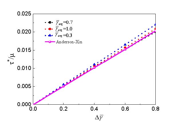
    [14] Anderson PM, Xin X (2000) The Critical Shear Stress to Transmit A Peierls Screw Dislocation Across A Non-slipping Interface. Multiscale Fracture and Deformationin Materials and Structures: The James R Rice 60th Anniversary Volume. Springer Netherland; 84: 87-105.
    [15] Anderson PM, Li Z (2001) A Peierls analysis of the critical stress fortransmission of a screw dislocation across a coherent, sliding interface. Mater Sci Eng A 319:182-187.
    [16] Shen Y, Anderson PM (2006) Transmission of a screw dislocation across acoherent, slipping interface. Acta Mater 54: 3941-3951.
    [17] Shen Y, Anderson PM (2007) Transmission of a screw dislocation across a coherent, non-slipping interface. J Mech Phys Solids 55: 956-979.
    [18] Chu HJ, Wang J, Beyerlein IJ, et al. (2013) Dislocation models of interfacial shearing induced by an approaching lattice glide dislocation. Int J Plast 41: 1-13.
    [19] Demkowicz MJ, Wang J, Hoagland RG (2008) Interfaces between dissimilar crystalline solids. Dislocations in Solids. Amsterdam: Elsevier North-Holland; 14: 141-205. doi: 10.1016/S1572-4859(07)00003-4
    [20] Rao SI, Hazzledine PM (2000) Atomistic simulations of dislocation-interface interactions in the Cu-Ni multilayer system. Phil Mag A 80: 2011-2040. doi: 10.1080/01418610008212148
    [21] Hoagland RG, Hirth JP, Misra A (2006) On the role of weak interfaces in blocking slip in nanoscale layered composites. Phil Mag 86: 3537-3558.
    [22] Wang J, Hoagland RG, Hirth JP, et al. (2008) Atomistic modeling of the interaction of glide dislocations with “weak” interfaces. Acta Mater 56: 5685-5693. doi: 10.1016/j.actamat.2008.07.041
    [23] Wang J, Hoagland RG, Hirth JP, et al. (2008) Atomistic simulations of the shear strength and sliding mechanisms of copper-niobium interfaces. Acta Mater 56: 3109-3119.
    [24] Wang J, Hoagland RG, Liu XY, et al. (2011) The influence of interface shear strength on the glide dislocation-interface interactions. Acta Mater 59: 3164-3173.
    [25] Wang J, Misra A, Hoagland RG, et al. (2012) Slip transmission across fcc/bcc interfaces with varying interface shear strengths. Acta Mater 60: 1503-13.
    [26] Zhu T, Li J, Samanta A, et al. (2007) Interfacial plasticity governs strain rate sensitivity and ductility in nanostructured metals. Proc Natl Acad Sci 104: 3031-3036.
    [27] Wang YU, Jin YM, Cuitino AM, et al. (2001) Nanoscale phase field microelasticity theory of dislocations: model and 3D simulations. Acta Mater 49:1847-1857.
    [28] Wang Y, Li J (2010) Phase field modeling of defects and deformation. Acta Mater 58: 1212-1235.
    [29] Shen C, Wang Y (2003) Phase field model of dislocation networks. Acta Mater 51: 2595-2610.
    [30] Shen C, Wang Y (2004) Incorporation of γ-surface to phase field model of dislocations: simulating dislocation dissociation in fcc crystals. Acta Mater 52: 683-691. doi: 10.1016/j.actamat.2003.10.014
    [31] Koslowski M, Cuitino AM, Ortiz M (2002) A phase-field theory of dislocation dynamics, strain hardening and hysteresis in ductile single crystals. J Mech Phys Solids 50: 2597-2635. doi: 10.1016/S0022-5096(02)00037-6
    [32] Hunter A, Beyerlein IJ, Germann TC, et al. (2011) Influence of the stacking fault energy surface on partial dislocations in fcc metals with a three-dimensional phase field dislocations dynamics model. Phys Rev B 84: 144108. doi: 10.1103/PhysRevB.84.144108
    [33] Koslowski M, Lee DW, Lei L (2011) Role of grain boundary energetics on the maximum strength of nanocrystalline Nickel. J Mech Phys Solids, 59: 1427-1436. doi: 10.1016/j.jmps.2011.03.011
    [34] Cao L, Hunter A, Beyerlein IJ, et al. (2015) The role of partial mediated slip during quasi-static deformation of 3D nanocrystalline metals. J Mech Phys Solids 78:415-426. doi: 10.1016/j.jmps.2015.02.019
    [35] Mianroodi JR, Svendsen B (2015) Atomistically determined phase-field modeling of dislocation dissociation, stacking fault formation, dislocation slip, and reactions in fcc systems. J Mech Phys Solids 77: 109-122. doi: 10.1016/j.jmps.2015.01.007
    [36] Zheng SL, Ni Y, He LH (2015) Phase field modeling of a glide dislocation transmission across a coherent sliding interface. Modelling Simul Mater Sci Eng 23: 035002.
    [37] Vitek V (1968) Intrinsic stacking faults in body-centred cubic crystals. Phil Mag 18: 773-786 doi: 10.1080/14786436808227500
    [38] Levitas VI, Javanbakht M (2012) Advanced phase-field approach to dislocation evolution. Phys.Rev B86: 140101.
    [39] Levitas VI, Javanbakht M (2013) Phase field approach to interaction of phase transformation and dislocation evolution. Appl Phys Lett 102: 251904.
    [40] Levitas VI, Javanbakht M (2014) Phase transformations in nanograin materials under high pressure and plastic shear: nanoscale mechanisms. Nanoscale 6: 162-166. doi: 10.1039/C3NR05044K
    [41] Levitas VI, Javanbakht M (2015) Thermodynamically consistent phase field approach to dislocation evolution at small and large strains. J Mech Phys Solids 82: 345-366. doi: 10.1016/j.jmps.2015.05.009
    [42] Levitas VI, Javanbakht M (2015) Interaction between phase transformations and dislocations at the nanoscale Part 1 General phase field approach. J Mech Phys Solids 82: 287-319. doi: 10.1016/j.jmps.2015.05.005
    [43] Levitas VI, Javanbakht M (2015) Interaction between phase transformations and dislocations at the nanoscale Part 2 Phase field simulation examples. J Mech Phys Solids 82: 164-185. doi: 10.1016/j.jmps.2015.05.006
    [44] Rice JR (1992) Dislocation nucleation from a crack tip: an analysis based on the Peierls concept. J Mech Phys Solids 40: 239-271. doi: 10.1016/S0022-5096(05)80012-2
    [45] Khachaturyan AG, Shatalov GA (1969) Elastic interaction potential of defects in a crystal. Sov Phys Solid State 11: 118-123.
    [46] Khachaturyan AG (1982) Theory of structural transformations in solids. New York: John Wiley & Sons.
  • This article has been cited by:

    1. Muqrin A. Almuqrin, A new flexible distribution with applications to engineering data, 2023, 69, 11100168, 371, 10.1016/j.aej.2023.01.046
    2. Mahdi Rasekhi, Mohammad Mehdi Saber, G. G Hamedani, M. M.Abd El-Raouf, Ramy Aldallal, Ahmed M. Gemeay, Melike Kaplan, Approximate Maximum Likelihood Estimations for the Parameters of the Generalized Gudermannian Distribution and Its Characterizations, 2022, 2022, 2314-4785, 1, 10.1155/2022/4092576
    3. Yinghui Zhou, Zubair Ahmad, Zahra Almaspoor, Faridoon Khan, Elsayed tag-Eldin, Zahoor Iqbal, Mahmoud El-Morshedy, On the implementation of a new version of the Weibull distribution and machine learning approach to model the COVID-19 data, 2022, 20, 1551-0018, 337, 10.3934/mbe.2023016
    4. Abdulaziz S. Alghamdi, M. M. Abd El-Raouf, A New Alpha Power Cosine-Weibull Model with Applications to Hydrological and Engineering Data, 2023, 11, 2227-7390, 673, 10.3390/math11030673
    5. Najwan Alsadat, Aijaz Ahmad, Muzamil Jallal, Ahmed M. Gemeay, Mohammed A. Meraou, Eslam Hussam, Ehab M.Elmetwally, Md. Moyazzem Hossain, The novel Kumaraswamy power Frechet distribution with data analysis related to diverse scientific areas, 2023, 70, 11100168, 651, 10.1016/j.aej.2023.03.003
    6. Najwan Alsadat, A new modified model with application to engineering data sets, 2023, 72, 11100168, 1, 10.1016/j.aej.2023.03.050
    7. Xiangming Tang, Jin-Taek Seong, Randa Alharbi, Aned Al Mutairi, Said G. Nasr, A new probabilistic model: Theory, simulation and applications to sports and failure times data, 2024, 10, 24058440, e25651, 10.1016/j.heliyon.2024.e25651
    8. Ibrahim Alkhairy, A new approach of generalized Rayleigh distribution with analysis of asymmetric data sets, 2024, 100, 11100168, 1, 10.1016/j.aej.2024.04.070
    9. Shahid Mohammad, Isabel Mendoza, A New Hyperbolic Tangent Family of Distributions: Properties and Applications, 2024, 2198-5804, 10.1007/s40745-024-00516-5
    10. Amulya Kumar Mahto, Yogesh Mani Tripathi, Sanku Dey, M.M. Abd El-Raouf, Najwan Alsadat, Efficient estimation of the density and distribution functions of Weibull-Burr XII distribution, 2024, 104, 11100168, 576, 10.1016/j.aej.2024.07.118
    11. Faridoon Khan, Zubair Ahmad, Saima K. Khosa, Mohammed Ahmed Alomair, Abdullah Mohammed Alomair, Abdulaziz khalid Alsharidi, A new modification of the flexible Weibull distribution based on power transformation: Monte Carlo simulation and applications, 2023, 9, 24058440, e17238, 10.1016/j.heliyon.2023.e17238
    12. Laxmi Prasad Sapkota, Vijay Kumar, Ahmed M. Gemeay, M. E. Bakr, Oluwafemi Samson Balogun, Abdisalam Hassan Muse, New Lomax-G family of distributions: Statistical properties and applications, 2023, 13, 2158-3226, 10.1063/5.0171949
    13. Xiaochun Liu, Jian Ji, Afaf Alrashidi, Fatimah A. Almulhim, Etaf Alshawarbeh, Jin-Taek Seong, A new probabilistic model with mixed-state failure rates: Modeling time-to-event scenarios in reliability and music engineering, 2024, 96, 11100168, 99, 10.1016/j.aej.2024.03.103
    14. M.M. Abd El-Raouf, Mohammed AbaOud, A novel extension of generalized Rayleigh model with engineering applications, 2023, 73, 11100168, 269, 10.1016/j.aej.2023.04.063
    15. Aijaz Ahmad, Najwan Alsadat, Mintodê Nicodème Atchadé, S. Qurat ul Ain, Ahmed M. Gemeay, Mohammed Amine Meraou, Ehab M. Almetwally, Md. Moyazzem Hossain, Eslam Hussam, New hyperbolic sine-generator with an example of Rayleigh distribution: Simulation and data analysis in industry, 2023, 73, 11100168, 415, 10.1016/j.aej.2023.04.048
    16. Zubir Shah, Ehab M. Almetwally, Dost Muhammad Khan, Farrukh Jamal, A novel odd Type-X family of distributions: Model, theory, and applications to medical, insurance, and engineering data sets, 2025, 18, 16878507, 101451, 10.1016/j.jrras.2025.101451
    17. Suleman Nasiru, Christophe Chesneau, Selasi Kwaku Ocloo, Abdul Ghaniyyu Abubakari, The Log-Cosine-Power Generated Family of Distributions, 2025, 2730-9657, 10.1007/s44007-025-00162-0
    18. Badr Aloraini, Improved estimation of population parameter of in the existence of nonresponse using auxiliary information, 2025, 10, 2473-6988, 12312, 10.3934/math.2025558
  • Reader Comments
  • © 2015 the Author(s), licensee AIMS Press. This is an open access article distributed under the terms of the Creative Commons Attribution License (http://creativecommons.org/licenses/by/4.0)
通讯作者: 陈斌, bchen63@163.com
  • 1. 

    沈阳化工大学材料科学与工程学院 沈阳 110142

  1. 本站搜索
  2. 百度学术搜索
  3. 万方数据库搜索
  4. CNKI搜索

Metrics

Article views(6051) PDF downloads(958) Cited by(0)

Figures and Tables

Figures(12)

Other Articles By Authors

/

DownLoad:  Full-Size Img  PowerPoint
Return
Return

Catalog