TikTok is a significant part of social media usage, since 25.6% of the total global population has a TikTok account, and, thus, scholars should pay attention to its association with users' mental health.
To synthesize and evaluate the association between problematic TikTok use and mental health.
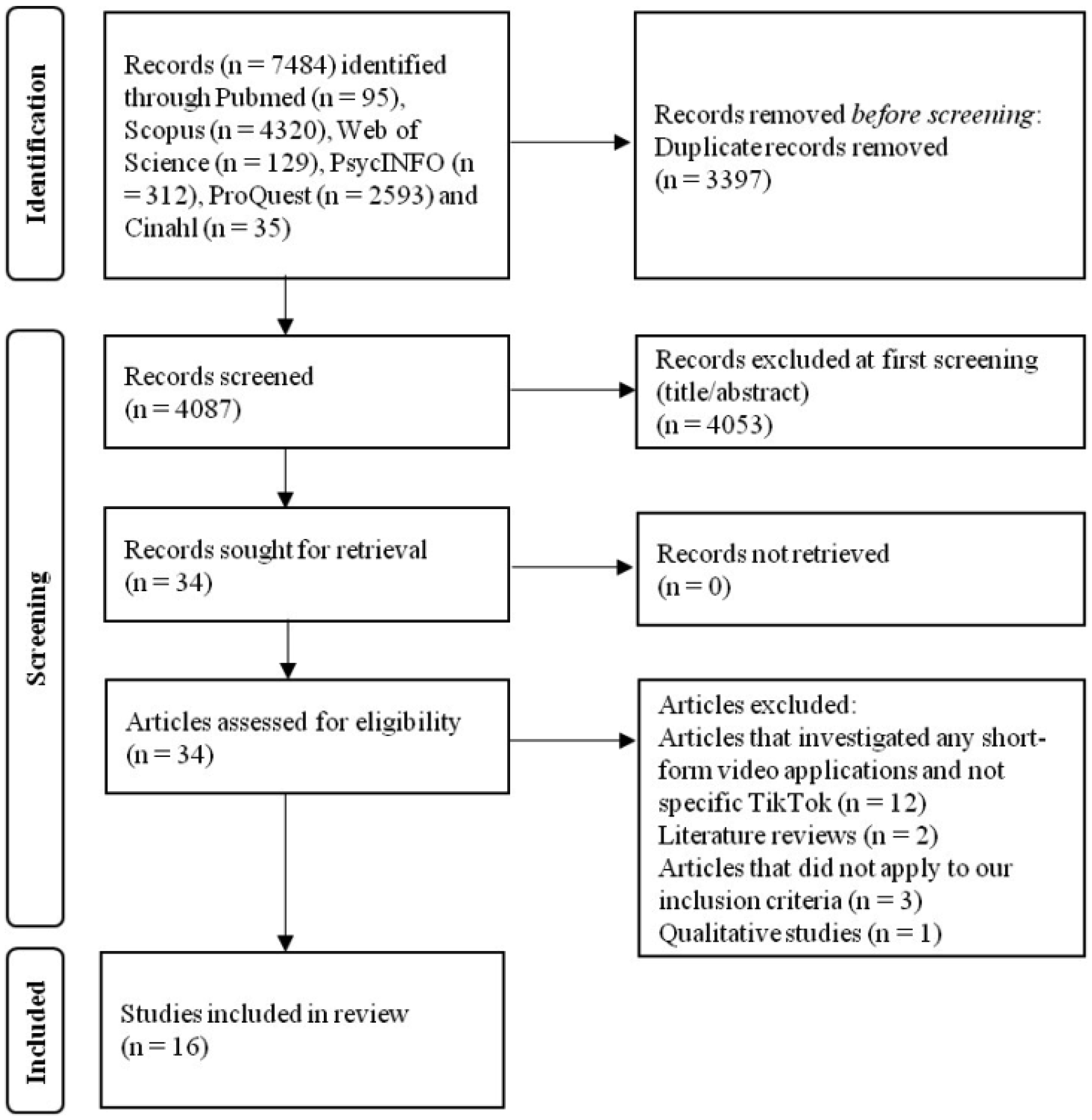
We applied the Preferred Reporting Items for Systematic Reviews and Meta-Analysis guidelines in our review. The review protocol was registered with PROSPERO (CRD42024582054). We searched PubMed, Scopus, Web of Science, PsycINFO, ProQuest, and CINAHL until September 02, 2024.
We identified 16 studies with 15,821 individuals. All studies were cross-sectional and were conducted after 2019. Quality was moderate in 10 studies, good in three studies, and poor in three studies. Our random effects models showed a positive association between TikTok use and depression (β = 0.321, 95% confidence interval: 0.261 to 0.381, p < 0.001, I2 = 78.0%, n = 6 studies), and anxiety (β = 0.406, 95% confidence interval: 0.279 to 0.533, p < 0.001, I2 = 94.8%, n = 4 studies). Data to perform meta-analysis with the other mental health variables were limited. However, our descriptive data showed a positive association between TikTok use and body image issues, poor sleep, anger, distress intolerance, narcissism, and stress.
Our findings suggest that problematic TikTok use has a negative association with several mental health issues. Given the high levels of TikTok use, especially among young adults, our findings are essential to further enhance our understanding of the association between TikTok use and mental health. Finally, there is a need for further studies of better quality to assess the association between problematic TikTok use and mental health in a more valid way.
Citation: Petros Galanis, Aglaia Katsiroumpa, Zoe Katsiroumpa, Polyxeni Mangoulia, Parisis Gallos, Ioannis Moisoglou, Evmorfia Koukia. Association between problematic TikTok use and mental health: A systematic review and meta-analysis[J]. AIMS Public Health, 2025, 12(2): 491-519. doi: 10.3934/publichealth.2025027
TikTok is a significant part of social media usage, since 25.6% of the total global population has a TikTok account, and, thus, scholars should pay attention to its association with users' mental health.
To synthesize and evaluate the association between problematic TikTok use and mental health.
We applied the Preferred Reporting Items for Systematic Reviews and Meta-Analysis guidelines in our review. The review protocol was registered with PROSPERO (CRD42024582054). We searched PubMed, Scopus, Web of Science, PsycINFO, ProQuest, and CINAHL until September 02, 2024.
We identified 16 studies with 15,821 individuals. All studies were cross-sectional and were conducted after 2019. Quality was moderate in 10 studies, good in three studies, and poor in three studies. Our random effects models showed a positive association between TikTok use and depression (β = 0.321, 95% confidence interval: 0.261 to 0.381, p < 0.001, I2 = 78.0%, n = 6 studies), and anxiety (β = 0.406, 95% confidence interval: 0.279 to 0.533, p < 0.001, I2 = 94.8%, n = 4 studies). Data to perform meta-analysis with the other mental health variables were limited. However, our descriptive data showed a positive association between TikTok use and body image issues, poor sleep, anger, distress intolerance, narcissism, and stress.
Our findings suggest that problematic TikTok use has a negative association with several mental health issues. Given the high levels of TikTok use, especially among young adults, our findings are essential to further enhance our understanding of the association between TikTok use and mental health. Finally, there is a need for further studies of better quality to assess the association between problematic TikTok use and mental health in a more valid way.

| [1] | StatistaSocial Media & User-generated content (2024). [cited 2025 February 01]. Available from: https://www.statista.com/statistics/278414/number-of-worldwide-social-network-users/ |
| [2] | BacklinkoTikTok statistics you need to know (2024). [cited 2025 February 01]. Available from: https://backlinko.com/tiktok-users |
| [3] |
Merchant RM, Lurie N (2020) Social media and emergency preparedness in response to novel coronavirus. JAMA 323: 2011-2012. https://doi.org/10.1001/jama.2020.4469 
|
| [4] |
Helm PJ, Jimenez T, Galgali MS, et al. (2022) Divergent effects of social media use on meaning in life via loneliness and existential isolation during the coronavirus pandemic. J Soc Pers Relat 39: 1768-1793. https://doi.org/10.1177/02654075211066922
|
| [5] |
Khan MN, Ashraf MA, Seinen D, et al. (2021) Social media for knowledge acquisition and dissemination: The impact of the COVID-19 pandemic on collaborative learning driven social media adoption. Front Psychol 12: 648253. https://doi.org/10.3389/fpsyg.2021.648253
|
| [6] |
Rosen AO, Holmes AL, Balluerka N, et al. (2022) Is social media a new type of social support? Social media use in spain during the COVID-19 pandemic: A mixed methods study. Int J Environ Res Public Health 19: 3952. https://doi.org/10.3390/ijerph19073952
|
| [7] |
Yang JZ, Liu Z, Wong JC (2022) Information seeking and information sharing during the COVID-19 pandemic. Commun Q 70: 1-21. https://doi.org/10.1080/01463373.2021.1995772
|
| [8] |
Szeto S, Au AKY, Cheng SKL (2024) Support from social media during the COVID-19 Pandemic: A systematic review. Behav Sci (Basel) 14: 759. https://doi.org/10.3390/bs14090759
|
| [9] |
Hmidan A, Seguin D, Duerden EG (2023) Media screen time use and mental health in school aged children during the pandemic. BMC Psychol 11: 202. https://doi.org/10.1186/s40359-023-01240-0
|
| [10] | Seguin D, Kuenzel E, Morton JB, et al. (2021) School's out: Parenting stress and screen time use in school-age children during the COVID-19 pandemic. J Affect Disord Rep 6: 100217. https://doi.org/10.1016/j.jadr.2021.100217 |
| [11] |
De Rosis S, Lopreite M, Puliga M, et al. (2021) The early weeks of the Italian Covid-19 outbreak: Sentiment insights from a Twitter analysis. Health Policy 125: 987-994. https://doi.org/10.1016/j.healthpol.2021.06.006
|
| [12] |
Lopreite M, Panzarasa P, Puliga M, et al. (2021) Early warnings of COVID-19 outbreaks across Europe from social media. Sci Rep 11: 2147. https://doi.org/10.1038/s41598-021-81333-1
|
| [13] |
Tsao SF, Chen H, Tisseverasinghe T, et al. (2021) What social media told us in the time of COVID-19: A scoping review. Lancet Digit Health 3: e175-e194. https://doi.org/10.1016/S2589-7500(20)30315-0
|
| [14] |
Haenlein M, Anadol E, Farnsworth T, et al. (2020) Navigating the new era of influencer marketing: How to be successful on Instagram, TikTok, & Co. Calif Manage Rev 63: 5-25. https://doi.org/10.1177/0008125620958166
|
| [15] | Pedrouzo S, Krynski L (2023) Hyperconnected: Children and adolescents on social media. The TikTok phenomenon. Arch Argent Pediatr 121: e202202674. https://doi.org/10.5546/aap.2022-02674.eng |
| [16] | Grandinetti J (2023) Examining embedded apparatuses of AI in Facebook and TikTok. AI & Soc 38: 1273-1286. https://doi.org/10.1007/s00146-021-01270-5 |
| [17] |
Kang H, Lou C (2022) AI agency vs. human agency: understanding human–AI interactions on TikTok and their implications for user engagement. J Comput-Mediat Comm 27: zmac014. https://doi.org/10.1093/jcmc/zmac014
|
| [18] |
Montag C, Yang H, Elhai JD (2021) On the psychology of TikTok use: A first glimpse from empirical findings. Front Public Health 9: 641673. https://doi.org/10.3389/fpubh.2021.641673
|
| [19] | TikTokMental and behavioral health (2024). [cited 2025 February 01]. Available from: https://www.tiktok.com/community-guidelines/en/mental-behavioral-health?lang=en |
| [20] |
Lookingbill V (2022) Examining nonsuicidal self-injury content creation on TikTok through qualitative content analysis. Libr Inform Sci Res 44: 101199. https://doi.org/10.1016/j.lisr.2022.101199
|
| [21] | Center for Countering Digital HateTikTok pushes harmful content promoting eating disorders and self-harm into users' feeds (2022). [cited 2025 February 01]. Available from: https://counterhate.com/research/deadly-by-design/ |
| [22] |
Karizat N, Delmonaco D, Eslami M, et al. (2021) Algorithmic folk theories and identity: How TikTok users co-produce knowledge of identity and engage in algorithmic resistance. Proc ACM Hum-Comput Interact 5: 1-44. https://doi.org/10.1145/3476046
|
| [23] |
Abbouyi S, Bouazza S, El Kinany S, et al. (2024) Depression and anxiety and its association with problematic social media use in the MENA region: A systematic review. Egypt J Neurol Psychiatry Neurosurg 60: 15. https://doi.org/10.1186/s41983-024-00793-0
|
| [24] |
Ahmed O, Walsh E, Dawel A, et al. (2024) Social media use, mental health and sleep: A systematic review with meta-analyses. J Affect Disord 367: 701-712. https://doi.org/10.1016/j.jad.2024.08.193
|
| [25] |
Alonzo R, Hussain J, Stranges S, et al. (2021) Interplay between social media use, sleep quality, and mental health in youth: A systematic review. Sleep Med Rev 56: 101414. https://doi.org/10.1016/j.smrv.2020.101414
|
| [26] |
Baker DA, Algorta GP (2016) The relationship between online social networking and depression: A systematic review of quantitative studies. Cyberpsychol Behav Soc Netw 19: 638-648. https://doi.org/10.1089/cyber.2016.0206
|
| [27] | Casale S, Banchi V (2020) Narcissism and problematic social media use: A systematic literature review. Addict Behav Rep 11: 100252. https://doi.org/10.1016/j.abrep.2020.100252 |
| [28] |
Marino C, Gini G, Vieno A, et al. (2018) The associations between problematic Facebook use, psychological distress and well-being among adolescents and young adults: A systematic review and meta-analysis. J Affect Disord 226: 274-281. https://doi.org/10.1016/j.jad.2017.10.007
|
| [29] |
Shannon H, Bush K, Villeneuve PJ, et al. (2022) Problematic social media use in adolescents and young adults: Systematic review and meta-analysis. JMIR Ment Health 9: e33450. https://doi.org/10.2196/33450
|
| [30] |
Wu W, Huang L, Yang F (2024) Social anxiety and problematic social media use: A systematic review and meta-analysis. Addict Behav 153: 107995. https://doi.org/10.1016/j.addbeh.2024.107995
|
| [31] |
Amin S, Iftikhar A, Meer A (2022) Intervening effects of academic performance between TikTok obsession and psychological wellbeing challenges in university students. Online Media Soc 3: 244-255. https://doi.org/10.71016/oms/qy5har60
|
| [32] |
Hendrikse C, Limniou M (2024) The use of Instagram and TikTok in relation to problematic use and well-Being. J Technol Behav Sci 9: 846-857. https://doi.org/10.1007/s41347-024-00399-6
|
| [33] |
Rogowska AM, Cincio A (2024) Procrastination mediates the relationship between problematic TikTok use and depression among young adults. J Clin Med 13: 1247. https://doi.org/10.3390/jcm13051247
|
| [34] |
Williams M, Lewin KM, Meshi D (2024) Problematic use of five different social networking sites is associated with depressive symptoms and loneliness. Curr Psychol 43: 20891-20898. https://doi.org/10.1007/s12144-024-05925-6
|
| [35] | Conte G, Iorio GD, Esposito D, et al. (2024) Scrolling through adolescence: A systematic review of the impact of TikTok on adolescent mental health. Eur Child Adolesc Psychiatry 16. https://doi.org/10.1007/s00787-024-02581-w |
| [36] |
Walker E, Hernandez AV, Kattan MW (2008) Meta-analysis: Its strengths and limitations. Cleve Clin J Med 75: 431-439. https://doi.org/10.3949/ccjm.75.6.431
|
| [37] |
Egger M, Smith GD, Phillips AN (1997) Meta-analysis: Principles and procedures. BMJ 315: 1533-1537. https://doi.org/10.1136/bmj.315.7121.1533
|
| [38] |
Finckh A, Tramèr MR (2008) Primer: strengths and weaknesses of meta-analysis. Nat Rev Rheumatol 4: 146-152. https://doi.org/10.1038/ncprheum0732
|
| [39] | Ioannidis JPA, Lau J (1999) Pooling research results: Benefits and limitations of meta-Analysis. Jt Comm J Qual Improv 25: 462-469. https://doi.org/10.1016/S1070-3241(16)30460-6 |
| [40] | Csikszentmihalyi M (2002) Flow: the classic work on how to achieve happiness. London, Rider: Random House. |
| [41] |
Montag C, Lachmann B, Herrlich M, et al. (2019) Addictive features of social media/messenger platforms and freemium games against the background of psychological and economic theories. Int J Environ Res Public Health 16: 2612. https://doi.org/10.3390/ijerph16142612
|
| [42] |
Andreassen CS, Billieux J, Griffiths MD, et al. (2016) The relationship between addictive use of social media and video games and symptoms of psychiatric disorders: A large-scale cross-sectional study. Psychol Addict Behav 30: 252-262. https://doi.org/10.1037/adb0000160
|
| [43] |
Andreassen CS, Torsheim T, Brunborg GS, et al. (2012) Development of a Facebook addiction scale. Psychol Rep 110: 501-517. https://doi.org/10.2466/02.09.18.PR0.110.2.501-517
|
| [44] | Griffiths M (2005) A ‘components' model of addiction within a biopsychosocial framework. J Subst Abuse 10: 191-197. https://doi.org/10.1080/14659890500114359 |
| [45] |
Sun Y, Zhang Y (2021) A review of theories and models applied in studies of social media addiction and implications for future research. Addict Behav 114: 106699. https://doi.org/10.1016/j.addbeh.2020.106699
|
| [46] |
Varona MN, Muela A, Machimbarrena JM (2022) Problematic use or addiction? A scoping review on conceptual and operational definitions of negative social networking sites use in adolescents. Addict Behav 134: 107400. https://doi.org/10.1016/j.addbeh.2022.107400
|
| [47] |
Alonso J, Liu Z, Evans-Lacko S, et al. (2018) Treatment gap for anxiety disorders is global: Results of the world mental health surveys in 21 countries. Depress Anxiety 35: 195-208. https://doi.org/10.1002/da.22711
|
| [48] | Kazdin AE (2000) Encyclopedia of psychology. Washington, DC: American Psychological Association 145-152. |
| [49] |
Carstens E, Moberg GP (2000) Recognizing pain and distress in laboratory animals. ILAR J 41: 62-71. https://doi.org/10.1093/ilar.41.2.62
|
| [50] | (2013) American Psychiatric AssociationDiagnostic and statistical manual of mental disorders: DSM-5. Washington: American Psychiatric Association 329-354. https://doi.org/10.1176/appi.books.9780890425596 |
| [51] | Della Sala S (2021) Encyclopedia of behavioral neuroscience. San Diego: Elsevier Science & Technology 552-557. |
| [52] |
Pavlova M, Latreille V (2019) Sleep disorders. Am J Med 132: 292-299. https://doi.org/10.1016/j.amjmed.2018.09.021
|
| [53] | Peplau LA, Perlman D (1982) Loneliness: A sourcebook of current theory, research and therapy. New York: Wiley 1-18. |
| [54] | Ellis L, Hoskin A, Ratnasingam M (2018) Handbook of social status correlates. US: Elsevier 1-14. |
| [55] |
Miller DN (2011) Life satisfaction. Encyclopedia of Child Behavior and Development . Boston, MA: Springer US 887-889. https://doi.org/10.1007/978-0-387-79061-9_1659
|
| [56] |
Huppert FA (2009) Psychological well-being: Evidence regarding its causes and consequences. Appl Psych Health Well 1: 137-164. https://doi.org/10.1111/j.1758-0854.2009.01008.x
|
| [57] |
Moher D, Shamseer L, Clarke M, et al. (2015) Preferred reporting items for systematic review and meta-analysis protocols (PRISMA-P) 2015 statement. Syst Rev 4: 1. https://doi.org/10.1186/2046-4053-4-1
|
| [58] |
Park CU, Kim HJ (2015) Measurement of inter-rater reliability in systematic review. Hanyang Med Rev 35: 44. https://doi.org/10.7599/hmr.2015.35.1.44
|
| [59] |
McHugh ML (2012) Interrater reliability: The kappa statistic. Biochem Med (Zagreb) 22: 276-282. https://doi.org/10.11613/BM.2012.031
|
| [60] | Santos WM dos, Secoli SR, Püschel VA de A (2018) The Joanna Briggs institute approach for systematic reviews. Rev Lat Am Enfermagem 26: e3074. https://doi.org/10.1590/1518-8345.2885.3074 |
| [61] |
Nieminen P (2022) Application of standardized regression coefficient in meta-analysis. BioMedInformatics 2: 434-458. https://doi.org/10.3390/biomedinformatics2030028
|
| [62] | Vittinghoff E (2005) Regression methods in biostatistics: Linear, logistic, survival, and repeated measures models. New York: Springer 65-82. |
| [63] |
Higgins J (2003) Measuring inconsistency in meta-analyses. BMJ 327: 557-560. https://doi.org/10.1136/bmj.327.7414.557
|
| [64] |
Wallace BC, Schmid CH, Lau J, et al. (2009) Meta-analyst: Software for meta-analysis of binary, continuous and diagnostic data. BMC Med Res Methodol 9: 80. https://doi.org/10.1186/1471-2288-9-80
|
| [65] |
Al-Garni AM, Alamri HS, Asiri WMA, et al. (2024) Social media use and sleep quality among secondary school students in Aseer region: A cross-sectional study. Int J Gen Med 17: 3093-3106. https://doi.org/10.2147/IJGM.S464457
|
| [66] | Asad K, Ali F, Awais M (2022) Personality traits, narcissism and TikTok addiction: A parallel mediation approach. Int J Media Inf Lit 7: 293-304. https://doi.org/10.13187/ijmil.2022.2.293 |
| [67] |
Sarman A, Tuncay S (2023) The relationship of Facebook, Instagram, Twitter, TikTok and WhatsApp/Telegram with loneliness and anger of adolescents living in Turkey: A structural equality model. J Pediatr Nurs 72: 16-25. https://doi.org/10.1016/j.pedn.2023.03.017
|
| [68] |
Sha P, Dong X (2021) Research on adolescents regarding the indirect effect of depression, anxiety, and stress between TikTok use disorder and memory loss. Int J Environ Res Public Health 18: 8820. https://doi.org/10.3390/ijerph18168820
|
| [69] | Yang Y, Adnan H, Sarmiti N (2023) The relationship between anxiety and TikTok addiction among university students in China: Mediated by escapism and use intensity. Int J Media Inf Lit 8: 458-464. https://doi.org/10.13187/ijmil.2023.2.458 |
| [70] |
Yao N, Chen J, Huang S, et al. (2023) Depression and social anxiety in relation to problematic TikTok use severity: The mediating role of boredom proneness and distress intolerance. Comput Hum Behav 145: 107751. https://doi.org/10.1016/j.chb.2023.107751
|
| [71] |
López-Gil JF, Chen S, Jiménez-López E, et al. (2023) Are the use and addiction to social networks associated with disordered eating among adolescents? Findings from the EHDLA study. Int J Ment Health Addict 22: 3775-3789. https://doi.org/10.1007/s11469-023-01081-3
|
| [72] |
Masciantonio A, Bourguignon D, Bouchat P, et al. (2021) Don't put all social network sites in one basket: Facebook, Instagram, Twitter, TikTok, and their relations with well-being during the COVID-19 pandemic. PLoS One 16: e0248384. https://doi.org/10.1371/journal.pone.0248384
|
| [73] |
Landa-Blanco M, García YR, Landa-Blanco AL, et al. (2024) Social media addiction relationship with academic engagement in university students: The mediator role of self-esteem, depression, and anxiety. Heliyon 10: e24384. https://doi.org/10.1016/j.heliyon.2024.e24384
|
| [74] |
Sagrera CE, Magner J, Temple J, et al. (2022) Social media use and body image issues among adolescents in a vulnerable Louisiana community. Front Psychiatry 13: 1001336. https://doi.org/10.3389/fpsyt.2022.1001336
|
| [75] |
Blackburn MR, Hogg RC (2024) #ForYou? the impact of pro-ana TikTok content on body image dissatisfaction and internalisation of societal beauty standards. PLoS One 19: e0307597. https://doi.org/10.1371/journal.pone.0307597
|
| [76] |
Nasidi QY, Norde AB, Dahiru JM, et al. (2024) Tiktok usage, social comparison, and self-esteem among the youth: Moderating role of gender. Galactica Media 6: 121-137. https://doi.org/10.46539/gmd.v6i2.467
|
| [77] |
Hartanto A, Quek FYX, Tng GYQ, et al. (2021) Does social media use increase depressive symptoms? A reverse causation perspective. Front Psychiatry 12: 641934. https://doi.org/10.3389/fpsyt.2021.641934
|
| [78] |
Van Zalk N (2016) Social anxiety moderates the links between excessive chatting and compulsive internet use. Cyberpsychology 10: 3. https://doi.org/10.5817/CP2016-3-3
|
| [79] |
Adams SK, Kisler TS (2013) Sleep quality as a mediator between technology-related sleep quality, depression, and anxiety. Cyberpsychol Behav Soc Netw 16: 25-30. https://doi.org/10.1089/cyber.2012.0157
|
| [80] | Liu S, Wing YK, Hao Y, et al. (2019) The associations of long-time mobile phone use with sleep disturbances and mental distress in technical college students: A prospective cohort study. Sleep 42. https://doi.org/10.1093/sleep/zsy213 |
| [81] |
Caplan SE (2002) Problematic internet use and psychosocial well-being: Development of a theory-based cognitive–behavioral measurement instrument. Comput Hum Behav 18: 553-575. https://doi.org/10.1016/S0747-5632(02)00004-3
|
| [82] | Sanders CE, Field TM, Diego M, et al. (2000) The relationship of Internet use to depression and social isolation among adolescents. Adolescence 35: 237-242. |
| [83] |
Davis RA (2001) A cognitive-behavioral model of pathological internet use. Comput Hum Behav 17: 187-195. https://doi.org/10.1016/S0747-5632(00)00041-8
|
| [84] |
Morahan-Martin J, Schumacher P (2003) Loneliness and social uses of the internet. Comput Hum Behav 19: 659-671. https://doi.org/10.1016/S0747-5632(03)00040-2
|
| [85] |
Kross E, Verduyn P, Demiralp E, et al. (2013) Facebook use predicts declines in subjective well-being in young adults. PLoS One 8: e69841. https://doi.org/10.1371/journal.pone.0069841
|
| [86] |
Chou HT, Edge N (2012) “They are happier and having better lives than I am”: The impact of using Facebook on perceptions of others' lives. Cyberpsychol Behav Soc Netw 15: 117-121. https://doi.org/10.1089/cyber.2011.0324
|
| [87] |
Sagioglou C, Greitemeyer T (2014) Facebook's emotional consequences: Why Facebook causes a decrease in mood and why people still use it. Comput Hum Behav 35: 359-363. https://doi.org/10.1016/j.chb.2014.03.003
|
| [88] |
Primack BA, Shensa A, Sidani JE, et al. (2017) Social media use and perceived social isolation among young adults in the U.S. Am J Prev Med 53: 1-8. https://doi.org/10.1016/j.amepre.2017.01.010
|
| [89] |
Tandoc EC, Ferrucci P, Duffy M (2015) Facebook use, envy, and depression among college students: Is facebooking depressing?. Comput Hum Behav 43: 139-146. https://doi.org/10.1016/j.chb.2014.10.053
|
| [90] |
Smith RH, Kim SH (2007) Comprehending envy. Psychol Bull 133: 46-64. https://doi.org/10.1037/0033-2909.133.1.46
|
| [91] |
Block JJ (2008) Issues for DSM-V: Internet addiction. Am J Psychiatry 165: 306-307. https://doi.org/10.1176/appi.ajp.2007.07101556
|
| [92] |
Morrison CM, Gore H (2010) The relationship between excessive internet use and depression: A questionnaire-based study of 1,319 young people and adults. Psychopathology 43: 121-126. https://doi.org/10.1159/000277001
|
| [93] |
Meier EP, Gray J (2014) Facebook photo activity associated with body image disturbance in adolescent girls. Cyberpsychol Behav Soc Netw 17: 199-206. https://doi.org/10.1089/cyber.2013.0305
|
| [94] |
Wang R, Yang F, Haigh MM (2017) Let me take a selfie: Exploring the psychological effects of posting and viewing selfies and groupies on social media. Telemat Inform 34: 274-283. https://doi.org/10.1016/j.tele.2016.07.004
|
| [95] |
O'Keeffe GS, Clarke-Pearson K (2011) The impact of social media on children, adolescents, and families. Pediatrics 127: 800-804. https://doi.org/10.1542/peds.2011-0054
|
| [96] |
Qin Y, Musetti A, Omar B (2023) Flow experience is a key factor in the likelihood of adolescents' problematic TikTok use: The moderating role of active parental mediation. Int J Environ Res Public Health 20: 2089. https://doi.org/10.3390/ijerph20032089
|
| [97] |
Qin Y, Omar B, Musetti A (2022) The addiction behavior of short-form video app TikTok: The information quality and system quality perspective. Front Psychol 13: 932805. https://doi.org/10.3389/fpsyg.2022.932805
|
| [98] |
Elhai JD, Yang H, Fang J, et al. (2020) Depression and anxiety symptoms are related to problematic smartphone use severity in Chinese young adults: Fear of missing out as a mediator. Addict Behav 101: 105962. https://doi.org/10.1016/j.addbeh.2019.04.020
|
| [99] |
Pan W, Mu Z, Zhao Z, et al. (2023) Female users' TikTok use and body image: Active versus passive use and social comparison processes. Cyberpsychol Behav Soc Netw 26: 3-10. https://doi.org/10.1089/cyber.2022.0169
|
| [100] |
Geng Y, Gu J, Wang J, et al. (2021) Smartphone addiction and depression, anxiety: The role of bedtime procrastination and self-control. J Affect Disord 293: 415-421. https://doi.org/10.1016/j.jad.2021.06.062
|
| [101] |
Feng Y, Meng D, Guo J, et al. (2022) Bedtime procrastination in the relationship between self-control and depressive symptoms in medical students: From the perspective of sex differences. Sleep Med 95: 84-90. https://doi.org/10.1016/j.sleep.2022.04.022
|
| [102] |
Ha JH, Kim SY, Bae SC, et al. (2007) Depression and Internet addiction in adolescents. Psychopathology 40: 424-430. https://doi.org/10.1159/000107426
|
| [103] |
LeBourgeois MK, Hale L, Chang AM, et al. (2017) Digital media and sleep in childhood and adolescence. Pediatrics 140: S92-S96. https://doi.org/10.1542/peds.2016-1758J
|
| [104] |
Zubair U, Khan MK, Albashari M (2023) Link between excessive social media use and psychiatric disorders. Ann Med Surg (Lond) 85: 875-878. https://doi.org/10.1097/MS9.0000000000000112
|
| [105] |
El Asam A, Samara M, Terry P (2019) Problematic internet use and mental health among British children and adolescents. Addict Behav 90: 428-436. https://doi.org/10.1016/j.addbeh.2018.09.007
|
| [106] |
Kuss D, Griffiths M, Karila L, et al. (2014) Internet addiction: A systematic review of epidemiological research for the last decade. Curr Pharm Des 20: 4026-4052. https://doi.org/10.2174/13816128113199990617
|
| [107] |
Fan R (2023) The impact of TikTok short videos on anxiety level of juveniles in Shenzhen China. Proceedings of the 2022 International Conference on Science Education and Art Appreciation (SEAA 2022) . Paris: Atlantis Press SARL 535-542. https://doi.org/10.2991/978-2-494069-05-3_66
|
| [108] | Mironica A, Popescu CA, George D, et al. (2024) Social media influence on body image and cosmetic surgery considerations: A systematic review. Cureus 16: e65626. https://doi.org/10.7759/cureus.65626 |
| [109] |
Vincente-Benito I, Ramírez-Durán MDV (2023) Influence of social media use on body image and well-being among adolescents and young adults: A systematic review. J Psychosoc Nurs Ment Health Serv 61: 11-18. https://doi.org/10.3928/02793695-20230524-02
|
| [110] |
Galanis P, Katsiroumpa A, Moisoglou I, et al. (2024) The TikTok addiction scale: Development and validation. AIMS Public Health 11: 1172-1197. https://doi.org/10.3934/publichealth.2024061
|
| [111] |
Kwon M, Kim DJ, Cho H, et al. (2013) The smartphone addiction scale: Development and validation of a short version for adolescents. PLoS One 8: e83558. https://doi.org/10.1371/journal.pone.0083558
|
| [112] |
Chen IH, Strong C, Lin YC, et al. (2020) Time invariance of three ultra-brief internet-related instruments: Smartphone Application-Based Addiction Scale (SABAS), Bergen Social Media Addiction Scale (BSMAS), and the nine-item Internet Gaming Disorder Scale- Short Form (IGDS-SF9) (Study Part B). Addict Behav 101: 105960. https://doi.org/10.1016/j.addbeh.2019.04.018
|
| [113] |
Luo T, Qin L, Cheng L, et al. (2021) Determination the cut-off point for the Bergen social media addiction (BSMAS): Diagnostic contribution of the six criteria of the components model of addiction for social media disorder. J Behav Addict 10: 281-290. https://doi.org/10.1556/2006.2021.00025
|
| [114] | Zarate D, Hobson BA, March E, et al. (2023) Psychometric properties of the Bergen social media addiction scale: An analysis using item response theory. Addict Behav Rep 17: 100473. https://doi.org/10.1016/j.abrep.2022.100473 |
| [115] |
Servidio R, Griffiths MD, Di Nuovo S, et al. (2023) Further exploration of the psychometric properties of the revised version of the Italian smartphone addiction scale–short version (SAS-SV). Curr Psychol 42: 27245-27258. https://doi.org/10.1007/s12144-022-03852-y
|
| [116] | Galanis P, Katsiroumpa A, Moisoglou I, et al. Determining an optimal cut-off point for TikTok addiction using the TikTok addiction scale. [Preprint] (2025). https://doi.org/10.21203/rs.3.rs-4782800/v1 |
 publichealth-12-02-027-s001.pdf publichealth-12-02-027-s001.pdf |
 |


Figures(3) / Tables(3)

Petros Galanis, Aglaia Katsiroumpa, Zoe Katsiroumpa, Polyxeni Mangoulia, Parisis Gallos, Ioannis Moisoglou, Evmorfia Koukia. Association between problematic TikTok use and mental health: A systematic review and meta-analysis[J]. AIMS Public Health, 2025, 12(2): 491-519. doi: 10.3934/publichealth.2025027


 DownLoad: