Hispanic ethnicity is associated with an increased risk for severe disease in children with COVID-19. Identifying underlying contributors to this disparity can lead to improved health care utilization and prevention strategies.
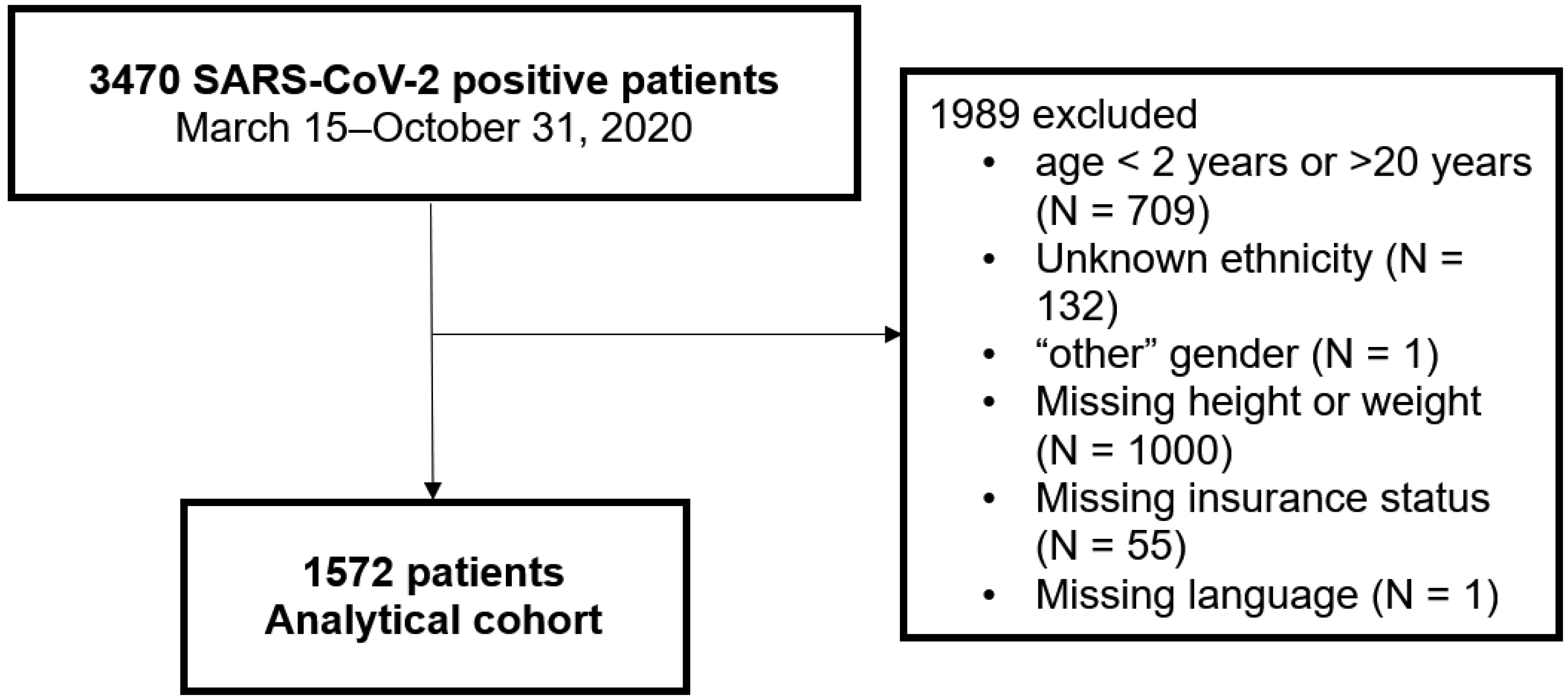
This is a retrospective cohort study of children 2–20 years of age with positive SARS-CoV-2 testing from March–October 2020. Univariable and multivariable logistic regression models were fitted to identify demographic, comorbid health conditions, and social vulnerabilities as predictors of severe COVID-19 (need for hospital admission or respiratory support).
We included 1572 children with COVID-19, of whom 45% identified as Hispanic. Compared to non-Hispanic children, patients who identified as Hispanic were more often obese (28% vs. 14%, p < 0.0001), preferred a non-English language (31% vs. 3%, p < 0.0001), and had Medicaid or no insurance (79% vs. 33%, p < 0.0001). In univariable analyses, children who identified as Hispanic were more likely to require hospital admission (OR 2.4, CI: 1.57–3.80) and respiratory support (OR 2.4, CI: 1.38–4.14). In multivariable analyses, hospital admission was associated with obesity (OR 1.9, CI: 1.15–3.08), non-English language (OR 2.4, CI: 1.35–4.23), and Medicaid insurance (OR 2.0, CI: 1.10–3.71), but ethnicity was not a significant predictor of severe disease.
The high rates of severe COVID-19 observed in Hispanic children early in the pandemic appeared to be secondary to underlying co-morbidities and social vulnerabilities that may have influenced access to care, such as language and insurance status. Pediatric providers and public health officials should tailor resource allocation to better target this underserved patient population.
Citation: Kelly Graff, Ye Ji Choi, Lori Silveira, Christiana Smith, Lisa Abuogi, Lisa Ross DeCamp, Jane Jarjour, Chloe Friedman, Meredith A. Ware, Jill L Kaar. Lessons learned for preventing health disparities in future pandemics: the role of social vulnerabilities among children diagnosed with severe COVID-19 early in the pandemic[J]. AIMS Public Health, 2025, 12(1): 124-136. doi: 10.3934/publichealth.2025009
Hispanic ethnicity is associated with an increased risk for severe disease in children with COVID-19. Identifying underlying contributors to this disparity can lead to improved health care utilization and prevention strategies.
This is a retrospective cohort study of children 2–20 years of age with positive SARS-CoV-2 testing from March–October 2020. Univariable and multivariable logistic regression models were fitted to identify demographic, comorbid health conditions, and social vulnerabilities as predictors of severe COVID-19 (need for hospital admission or respiratory support).
We included 1572 children with COVID-19, of whom 45% identified as Hispanic. Compared to non-Hispanic children, patients who identified as Hispanic were more often obese (28% vs. 14%, p < 0.0001), preferred a non-English language (31% vs. 3%, p < 0.0001), and had Medicaid or no insurance (79% vs. 33%, p < 0.0001). In univariable analyses, children who identified as Hispanic were more likely to require hospital admission (OR 2.4, CI: 1.57–3.80) and respiratory support (OR 2.4, CI: 1.38–4.14). In multivariable analyses, hospital admission was associated with obesity (OR 1.9, CI: 1.15–3.08), non-English language (OR 2.4, CI: 1.35–4.23), and Medicaid insurance (OR 2.0, CI: 1.10–3.71), but ethnicity was not a significant predictor of severe disease.
The high rates of severe COVID-19 observed in Hispanic children early in the pandemic appeared to be secondary to underlying co-morbidities and social vulnerabilities that may have influenced access to care, such as language and insurance status. Pediatric providers and public health officials should tailor resource allocation to better target this underserved patient population.
coronavirus disease 2019
severe acute respiratory syndrome coronavirus-2
Children's Hospital Colorado
Children and COVID-19 in Colorado study
electronic health record
social determinants of health
body mass index
Centers for Disease Control and Prevention
nonalcoholic fatty liver disease
nonalcoholic steatohepatitis
socioeconomic status

| [1] | American Academy of PediatricsChildren and COVID-19: State-Level Data Report (2022). Available from: https://downloads.aap.org/AAP/PDF/AAP%20and%20CHA%20-%20Children%20and%20COVID-19%20State%20Data%20Report%209.24.20%20FINAL.pdf |
| [2] | Centers for Disease Control and PreventionCOVID Data Tracker (2023). Available from: https://covid.cdc.gov/covid-data-tracker/?CDC_#datatracker-home |
| [3] |
Townsend MJ, Kyle TK, Stanford FC (2020) Outcomes of COVID-19: disparities in obesity and by ethnicity/race. Int J Obes 44: 1807-1809. https://doi.org/10.1038/s41366-020-0635-2 
|
| [4] |
Woo Baidal JA, Chang J, Hulse E, et al. (2020) Zooming Toward a Telehealth Solution for Vulnerable Children with Obesity During Coronavirus Disease 2019. Obesity 28: 1184-1186. https://doi.org/10.1002/oby.22860
|
| [5] |
Zachariah P, Johnson CL, Halabi KC, et al. (2020) Epidemiology, Clinical Features, and Disease Severity in Patients With Coronavirus Disease 2019 (COVID-19) in a Children's Hospital in New York City, New York. JAMA Pediatr 174: e202430. https://doi.org/10.1001/jamapediatrics.2020.2430
|
| [6] |
Graff K, Smith C, Silveira L, et al. (2021) Risk Factors for Severe COVID-19 in Children. Pediatr Infect Dis J 40: e137-e145. https://doi.org/10.1097/INF.0000000000003043
|
| [7] |
Hobbs CV, Woodworth K, Young CC, et al. (2022) Frequency, Characteristics and Complications of COVID-19 in Hospitalized Infants. Pediatr Infect Dis J 41: e81-e86. https://doi.org/10.1097/INF.0000000000003435
|
| [8] |
Woodruff RC, Campbell AP, Taylor CA, et al. (2021) Risk Factors for Severe COVID-19 in Children. Pediatrics 149: e2021053418. https://doi.org/10.1542/peds.2021-053418
|
| [9] |
Acosta AM, Garg S, Pham H, et al. (2021) Racial and Ethnic Disparities in Rates of COVID-19-Associated Hospitalization, Intensive Care Unit Admission, and In-Hospital Death in the United States From March 2020 to February 2021. JAMA Netw Open 4: e2130479. https://doi.org/10.1001/jamanetworkopen.2021.30479
|
| [10] |
Goyal MK, Simpson JN, Boyle MD, et al. (2020) Racial and/or Ethnic and Socioeconomic Disparities of SARS-CoV-2 Infection Among Children. Pediatrics 146: e2020009951. https://doi.org/10.1542/peds.2020-009951
|
| [11] |
Saatci D, Ranger TA, Garriga C, et al. (2021) Association Between Race and COVID-19 Outcomes Among 2.6 Million Children in England. JAMA Pediatr 175: 928-938. https://doi.org/10.1001/jamapediatrics.2021.1685
|
| [12] |
Smith C, Odd D, Harwood R, et al. (2022) Deaths in children and young people in England after SARS-CoV-2 infection during the first pandemic year. Nat Med 28: 185-192. https://doi.org/10.1038/s41591-021-01578-1
|
| [13] |
Vahidy FS, Nicolas JC, Meeks JR, et al. (2020) Racial and ethnic disparities in SARS-CoV-2 pandemic: analysis of a COVID-19 observational registry for a diverse US metropolitan population. BMJ Open 10: e039849. https://doi.org/10.1136/bmjopen-2020-039849
|
| [14] | Centers for Disease Control and PreventionCOVID-NET: Laboratory-Confirmed COVID-19-Associated Hospitalizations (2023). Available from: https://www.cdc.gov/mmwr/volumes/71/wr/mm7134a3.htm |
| [15] |
Romano SD, Blackstock AJ, Taylor EV, et al. (2021) Trends in Racial and Ethnic Disparities in COVID-19 Hospitalizations, by Region - United States, March–December 2020. MMWR Morb Mortal Wkly Rep 70: 560-565. https://doi.org/10.15585/mmwr.mm7015e2
|
| [16] |
Wong MS, Haderlein TP, Yuan AH, et al. (2021) Time Trends in Racial/Ethnic Differences in COVID-19 Infection and Mortality. Int J Environ Res Public Health 18: 4848. https://doi.org/10.3390/ijerph18094848
|
| [17] | O'Brien SC, Cole LD, Albanese BA, et al. (2023) SARS-CoV-2 Seroprevalence Compared with Confirmed COVID-19 Cases among Children, Colorado, USA, May–July 2021. Emerg Infect Dis 29: 929-936. https://doi.org/10.3201/eid2905.221541 |
| [18] | United States Census BureauU.S. Census Bureau Quick Facts (2022). Available from: https://www.census.gov/quickfacts/CO |
| [19] | Federal Interagency Forum on Child and Family StatisticsAmerica's Children: Key National Indicators of Well-Being, 2021 (2022). Available from: https://www.childstats.gov/pdf/ac2021/ac_21.pdf |
| [20] |
Gordon-Larsen P, Harris KM, Ward DS, et al. (2003) Acculturation and overweight-related behaviors among Hispanic immigrants to the US: the National Longitudinal Study of Adolescent Health. Soc Sci Med 57: 2023-2034. https://doi.org/10.1016/S0277-9536(03)00072-8
|
| [21] | NCLRToward A More Equitable Future: The Trends and Challenges Facing America's Latino Children (2016). Available from: https://unidosus.org/publications/1627-toward-a-more-equitable-future-the-trends-and-challenges-facing-americas-latino-children/ |
| [22] |
Ogden CL, Carroll MD, Kit BK, et al. (2012) Prevalence of obesity and trends in body mass index among US children and adolescents, 1999–2010. JAMA 307: 483-490. https://doi.org/10.1001/jama.2012.40
|
| [23] |
Skinner AC, Perrin EM, Skelton JA (2016) Prevalence of obesity and severe obesity in US children, 1999–2014. Obesity 24: 1116-1123. https://doi.org/10.1002/oby.21497
|
| [24] |
Tsankov BK, Allaire JM, Irvine MA, et al. (2021) Severe COVID-19 Infection and Pediatric Comorbidities: A Systematic Review and Meta-Analysis. Int J Infect Dis 103: 246-256. https://doi.org/10.1016/j.ijid.2020.11.163
|
| [25] |
Zhang F, Xiong Y, Wei Y, et al. (2020) Obesity predisposes to the risk of higher mortality in young COVID-19 patients. J Med Virol 92: 2536-2542. https://doi.org/10.1002/jmv.26039
|
| [26] |
Tripathi S, Christison AL, Levy E, et al. (2021) The Impact of Obesity on Disease Severity and Outcomes Among Hospitalized Children With COVID-19. Hosp Pediatr 11: e297-e316. https://doi.org/10.1542/hpeds.2021-006087
|
| [27] | Colorado CsH2015 Executive Summary: Community Health Needs Assessment (2015). Available from: https://www.richd.org/docs/communityhealth/AppendixA.pdf |
| [28] |
Harris PA, Taylor R, Thielke R, et al. (2009) Research electronic data capture (REDCap)--a metadata-driven methodology and workflow process for providing translational research informatics support. J Biomed Inform 42: 377-381. https://doi.org/10.1016/j.jbi.2008.08.010
|
| [29] |
Gulati AK, Kaplan DW, Daniels SR (2012) Clinical tracking of severely obese children: a new growth chart. Pediatrics 130: 1136-1140. https://doi.org/10.1542/peds.2012-0596
|
| [30] | CDC| BMIChild and Teen BMI categories (2022). Available from: https://www.cdc.gov/bmi/child-teen-calculator/bmi-categories.html |
| [31] |
Hernandez DC, Kimbro RT (2013) The association between acculturation and health insurance coverage for immigrant children from socioeconomically disadvantaged regions of origin. J Immigr Minor Health 15: 453-461. https://doi.org/10.1007/s10903-012-9643-1
|
| [32] |
Choy B, Arunachalam K, Gupta S, et al. (2021) Systematic review: Acculturation strategies and their impact on the mental health of migrant populations. Public Health Pract 2: 100069. https://doi.org/10.1016/j.puhip.2020.100069
|
| [33] |
DeLaroche AM, Rodean J, Aronson PL, et al. (2021) Pediatric Emergency Department Visits at US Children's Hospitals During the COVID-19 Pandemic. Pediatrics 147: e2020039628. https://doi.org/10.1542/peds.2020-039628
|
| [34] |
Fritz CQ, Fleegler EW, DeSouza H, et al. (2022) Child Opportunity Index and Changes in Pediatric Acute Care Utilization in the COVID-19 Pandemic. Pediatrics 149: e2021053706. https://doi.org/10.1542/peds.2021-053706
|
| [35] | Chen KL, Brozen M, Rollman JE, et al. (2021) How is the COVID-19 pandemic shaping transportation access to health care?. Transp Res Interdiscip Perspect 10: 100338. https://doi.org/10.1016/j.trip.2021.100338 |
| [36] |
Macy ML, Smith TL, Cartland J, et al. (2021) Parent-reported hesitancy to seek emergency care for children at the crest of the first wave of COVID-19 in Chicago. Acad Emerg Med 28: 355-358. https://doi.org/10.1111/acem.14214
|
 publichealth-12-01-009-s001.pdf publichealth-12-01-009-s001.pdf |
 |
Figures(1) / Tables(4)

Kelly Graff, Ye Ji Choi, Lori Silveira, Christiana Smith, Lisa Abuogi, Lisa Ross DeCamp, Jane Jarjour, Chloe Friedman, Meredith A. Ware, Jill L Kaar. Lessons learned for preventing health disparities in future pandemics: the role of social vulnerabilities among children diagnosed with severe COVID-19 early in the pandemic[J]. AIMS Public Health, 2025, 12(1): 124-136. doi: 10.3934/publichealth.2025009


 DownLoad: