Risk factors for severe dysmenorrhea in Arab women: A focus on war displacement and mental health outcomes

Omar Gammoh; Osama Abo Al Rob; Abdelrahim Alqudah; Ahmed Al-Smadi; Mohamad Obada Dobain; Reham Zeghoul; Alaa A. A. Aljabali; Mervat Alsous; Omar Gammoh; Osama Abo Al Rob; Abdelrahim Alqudah; Ahmed Al-Smadi; Mohamad Obada Dobain; Reham Zeghoul; Alaa A. A. Aljabali; Mervat Alsous

doi:10.3934/publichealth.2024010

AIMS Public Health

2024, Volume 11, Issue 1: 209-222. doi: 10.3934/publichealth.2024010

Previous Article Next Article

Research article

Risk factors for severe dysmenorrhea in Arab women: A focus on war displacement and mental health outcomes

1.
Department of Clinical Pharmacy and Pharmacy Practice, Faculty of Pharmacy, Yarmouk University, Irbid, 21163, Jordan
2.
Department of Clinical Pharmacy and Pharmacy Practice, Faculty of Pharmaceutical Sciences, The Hashemite University, Zarqa 13133, Jordan
3.
Adult Health Nursing, Prince Salma College, Al Al-Bayt University, Mafraq, Jordan
4.
Souriyat Across Borders, Amman, Jordan
5.
Department of Pharmaceutics and Pharmaceutical Technology, Faculty of Pharmacy, Yarmouk University, Irbid 21163, Jordan

Received: 26 October 2023 Revised: 26 January 2024 Accepted: 19 February 2024 Published: 26 February 2024

Background
Dysmenorrhea is wide spread gynecological disorder among that affect the quality of life of women world wide. The current study aims to examine whether war displacement, mental health symptoms, and other clinical factors are associated with dysmenorrhea severity.

Methods
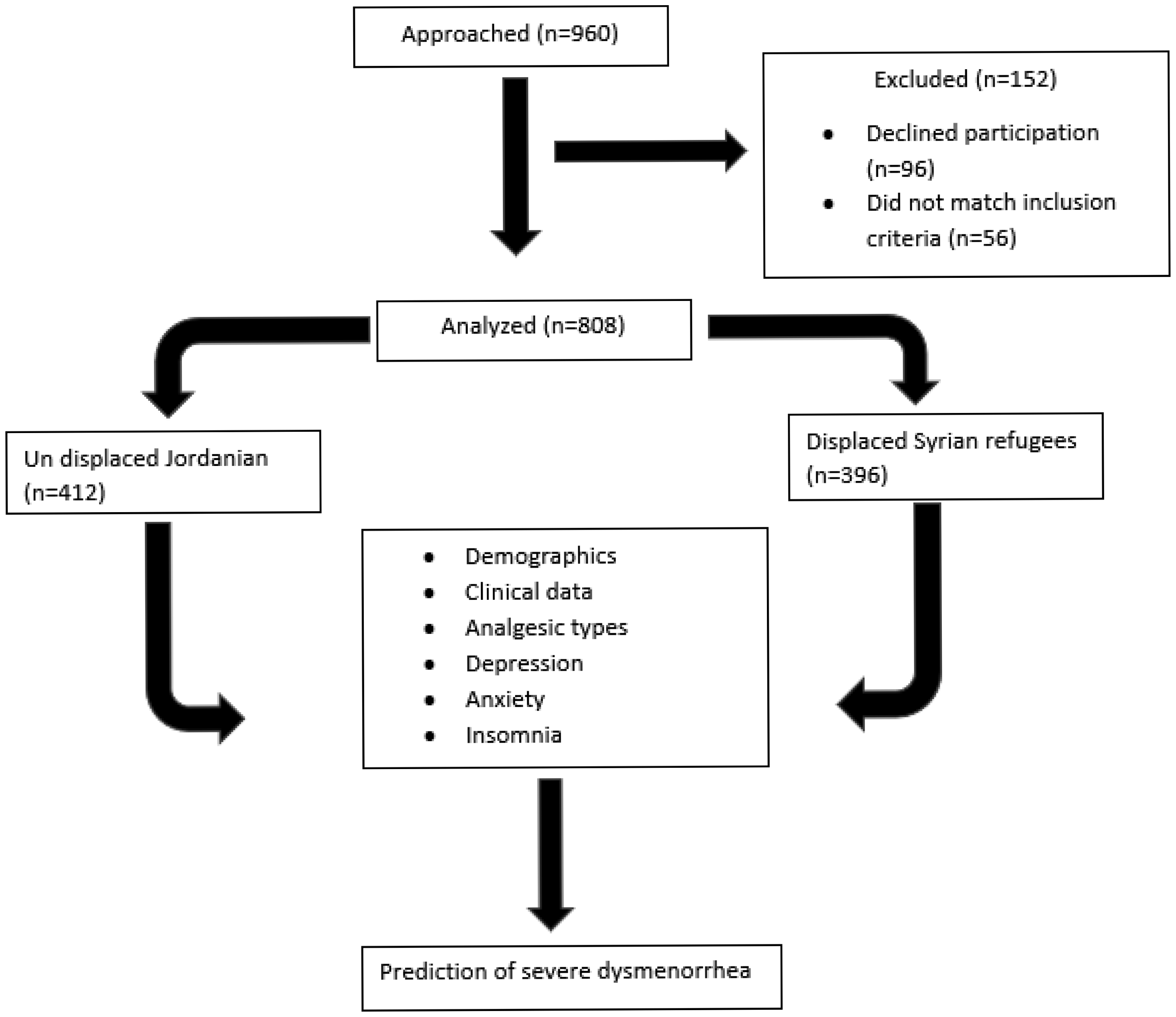
This is a cross-sectional case-control study recruiting two groups: displaced Syrian women and un-displaced local Jordanian women. Demographics and clinical details were recorded. The severity of dysmenorrhea was assessed using WaLIDD scale, the PHQ-9 scale was emplyed to assess depressive symptoms, anxiety was assessed using the GAD-7 scale, and insomnia was assessed using the ISI-A scale. Predictors of severe dysmenorrhea in females using multivariate binary logistic regression.

Results
Out of 808 of the total participants, 396 (49%) were Syrian displaced war refugees, 424 (42.5%) reported using paracetamol, 232 (23.2%) were using NSAIDs, and 257 (25.9%) using herbal remedies. Severe dysmenorrhea was associated with war displacement (OR = 2.14, 95% CI = 1.49–3.08, p < 0.001), not using NSAIDs (OR = 2.75, 95% CI = 1.91–3.95, p < 0.001), not using herbal remedies (OR = 2.01, 95% CI = 1.13–3.60, p = 0.01), depression (OR = 2.14, 95% CI = 1.40–3.29, p < 0.001), and insomnia (OR = 1.66, 95% CI = 1.14–2.42, p = 0.009).

Conclusions
War displacement, type of analgesic, depression, and insomnia are risk factors for severe dysmenorrhea.
- women,
- dysmenorrhea,
- war displacement,
- depression,
- anxiety,
- and insomnia
Citation: Omar Gammoh, Osama Abo Al Rob, Abdelrahim Alqudah, Ahmed Al-Smadi, Mohamad Obada Dobain, Reham Zeghoul, Alaa A. A. Aljabali, Mervat Alsous. Risk factors for severe dysmenorrhea in Arab women: A focus on war displacement and mental health outcomes[J]. AIMS Public Health, 2024, 11(1): 209-222. doi: 10.3934/publichealth.2024010

Related Papers:

Abstract

Background

Dysmenorrhea is wide spread gynecological disorder among that affect the quality of life of women world wide. The current study aims to examine whether war displacement, mental health symptoms, and other clinical factors are associated with dysmenorrhea severity.

Methods

This is a cross-sectional case-control study recruiting two groups: displaced Syrian women and un-displaced local Jordanian women. Demographics and clinical details were recorded. The severity of dysmenorrhea was assessed using WaLIDD scale, the PHQ-9 scale was emplyed to assess depressive symptoms, anxiety was assessed using the GAD-7 scale, and insomnia was assessed using the ISI-A scale. Predictors of severe dysmenorrhea in females using multivariate binary logistic regression.

Results

Out of 808 of the total participants, 396 (49%) were Syrian displaced war refugees, 424 (42.5%) reported using paracetamol, 232 (23.2%) were using NSAIDs, and 257 (25.9%) using herbal remedies. Severe dysmenorrhea was associated with war displacement (OR = 2.14, 95% CI = 1.49–3.08, p < 0.001), not using NSAIDs (OR = 2.75, 95% CI = 1.91–3.95, p < 0.001), not using herbal remedies (OR = 2.01, 95% CI = 1.13–3.60, p = 0.01), depression (OR = 2.14, 95% CI = 1.40–3.29, p < 0.001), and insomnia (OR = 1.66, 95% CI = 1.14–2.42, p = 0.009).

Conclusions

War displacement, type of analgesic, depression, and insomnia are risk factors for severe dysmenorrhea.

Acknowledgments

The authors would like to thank Caritas team in Jordan for facilitating this work. Also, special thanks to Prof. Giuseppe Moscati, Nour, Suzi, Sama and Yasmina.
This study was funded by Yarmouk University.

Conflict of Interest

The authors declare no conflicts of interest.
“The study was conducted in accordance with the Declaration of Helsinki, and approved by the Institutional Review Board (or Ethics Committee) of Yarmouk University (39/2022).
Informed consent was obtained from all subjects involved in the study. Written informed consent has been obtained from the patient(s) to publish this paper.
Data is available from the corresponding author and can be provided upon request.

References

[1]	Ferries-Rowe E, Corey E, Archer JS (2020) Primary dysmenorrhea: Diagnosis and therapy. Obstet Gynecol 136: 1047-1058. https://doi.org/10.1097/AOG.0000000000004096
[2]	De Sanctis V, Soliman AT, Elsedfy H, et al. (2016) Dysmenorrhea in adolescents and young adults: A review in different countries. Acta Biomed 87: 233-246.
[3]	Al-Husban N, Odeh O, Dabit T, et al. (2022) The influence of lifestyle variables on primary dysmenorrhea: A cross-sectional study. Int J Womens. Health 14: 545-553. https://doi.org/10.2147/IJWH.S338651
[4]	Al-Jefout M, Seham AF, Jameel H, et al. (2015) Dysmenorrhea: Prevalence and impact on quality of life among young adult Jordanian females. J Pediatr Adolesc Gynecol 28: 173-18. https://doi.org/10.1016/j.jpag.2014.07.005
[5]	Molla A, Duko B, Girma B, et al. (2022) Prevalence of dysmenorrhea and associated factors among students in Ethiopia: A systematic review and meta-analysis. Womens Heal 18: 17455057221079444. https://doi.org/10.1177/17455057221079443
[6]	Pakpour AH, Kazemi F, Alimoradi Z, et al. (2020) Depression, anxiety, stress, and dysmenorrhea: A protocol for a systematic review. Syst Rev 9: 65. https://doi.org/10.1186/s13643-020-01319-4
[7]	Proctor M, Farquhar C (2006) Diagnosis and management of dysmenorrhoea. BMJ 332: 1134-1138. https://doi.org/10.1136/bmj.332.7550.1134
[8]	Itani R, Soubra L, Karout S, et al. (2022) Primary dysmenorrhea: Pathophysiology, diagnosis, and treatment updates. Korean J Fam Med 43: 101-108. https://doi.org/10.4082/kjfm.21.0103
[9]	Agarwal AK, Agarwal A (2010) A study of dysmenorrhea during menstruation in adolescent girls. Indian J Community Med 35: 159-164. https://doi.org/10.4103/0970-0218.62586
[10]	Matthewman G, Lee A, Kaur JG, et al. (2018) Physical activity for primary dysmenorrhea: A systematic review and meta-analysis of randomized controlled trials. Am J Obstet Gynecol 219: 255e1-255e20. https://doi.org/10.1016/j.ajog.2018.04.001
[11]	Latthe P, Mignini L, Gray R, et al. (2006) Factors predisposing women to chronic pelvic pain: Systematic review. BMJ 332: 749-755. https://doi.org/10.1136/bmj.38748.697465.55
[12]	Takeda T, Tadakawa M, Koga S, et al. (2013) Relationship between dysmenorrhea and posttraumatic stress disorder in Japanese high school students 9 months after the Great East Japan Earthquake. J Pediatr Adolesc Gynecol 26: 355-357. https://doi.org/10.1016/j.jpag.2013.06.020
[13]	Gammouh OS, Al-Smadi AM, Tawalbeh LI, et al. (2015) Peer reviewed: Chronic diseases, lack of medications, and depression among Syrian refugees in Jordan, 2013–2014. Prev Chronic Dis 12: E10. https://doi.org/10.5888/pcd12.140424
[14]	Al-Smadi A M, Halaseh H J, Gammoh O S, et al. (2016) Do chronic diseases and availability of medications predict post-traumatic stress disorder (PTSD) among Syrian refugees in Jordan?. Pak J Nutr 15: 10, 936-941. https://doi.org/10.3923/pjn.2016.936.941
[15]	Sharghi M, Mansurkhani SM, Larky DA, et al. (2019) An update and systematic review on the treatment of primary dysmenorrhea. JBRA Assist Reprod 23: 51-57. https://doi.org/10.5935/1518-0557.20180083
[16]	Farotimi A A, Esike J, Nwozichi C U, et al. (2015) Knowledge, attitude, and healthcare-seeking behavior towards dysmenorrhea among female students of a private university in Ogun State, Nigeria. J Basic Clin Reprod Sci 4: 33-38. https://doi.org/10.4103/2278-960X.153524
[17]	Nie W, Xu P, Hao C, et al. (2020) Efficacy and safety of over-the-counter analgesics for primary dysmenorrhea: a network meta-analysis. Medicine (Baltimore) 99: e19881. https://doi.org/10.1097/MD.0000000000019881
[18]	Kokjohn K, Schmid D M, Triano J J, et al. (1992) The effect of spinal manipulation on pain and prostaglandin levels in women with primary dysmenorrhea. J Manipulative Physiol Ther 15: 279-285.
[19]	Castellsague J, Riera-Guardia N, Calingaert B, et al. (2012) Individual NSAIDs and upper gastrointestinal complications: A systematic review and meta-analysis of observational studies (the SOS project). Drug Saf 35: 1127-1146. https://doi.org/10.1007/BF03261999
[20]	Fanelli A, Romualdi P, Vigano' R, et al. (2013) Non-selective non-steroidal anti-inflammatory drugs (NSAIDs) and cardiovascular risk. Acta Biomed 84: 5-11.
[21]	Feng X, Wang X (2018) Comparison of the efficacy and safety of non-steroidal anti-inflammatory drugs for patients with primary dysmenorrhea: A network meta-analysis. Mol Pain 14: 1744806918770320. https://doi.org/10.1177/1744806918770320
[22]	Taherian AA, Babaei M, Vafaei AA, et al. (2009) Antinociceptive effects of hydroalcoholic extract of thymus vulgaris. Pak J Pharm Sci 22: 83-89.
[23]	Lim TK (2012) Edible medicinal and non-medicinal plants. The Netherlands: Springer 361-416. https://doi.org/10.1007/978-94-007-2534-8
[24]	Gammoh O, Durand H, Abu-Shaikh H, et al. (2023) Post-traumatic stress disorder burden among female Syrian war refugees is associated with dysmenorrhea severity but not with the analgesics. Electron J Gen Med 20: em485. https://doi.org/10.29333/ejgm/13089
[25]	Kroenke K, Spitzer RL, Williams JBW (2001) The PHQ-9. J Gen Intern Med 16: 606-613. https://doi.org/10.1046/j.1525-1497.2001.016009606.x
[26]	Sawaya H, Atoui M, Hamadeh A, et al. (2016) Adaptation and initial validation of the Patient Health Questionnaire-9 (PHQ-9) and the Generalized Anxiety Disorder-7 Questionnaire (GAD-7) in an Arabic speaking Lebanese psychiatric outpatient sample. Psychiatry Res 239: 245-252. https://doi.org/10.1016/j.psychres.2016.03.030
[27]	AlHadi AN, AlAteeq DA, Al-Sharif E, et al. (2017) An arabic translation, reliability, and validation of Patient Health Questionnaire in a Saudi sample. Ann Gen Psychiatry 16: 32. https://doi.org/10.1186/s12991-017-0155-1
[28]	Löwe B, Decker O, Müller S, et al. (2008) Validation and standardization of the Generalized Anxiety Disorder Screener (GAD-7) in the general population. Med Care 46: 266-274. https://doi.org/10.1097/MLR.0b013e318160d093
[29]	Morin C Insomnia: Psychological assessment and management (1993). Available from: https://psycnet.apa.org/record/1993-98362-000
[30]	Suleiman KH, Yates BC (2011) Translating the insomnia severity index into Arabic. J Nurs Scholarsh 43: 49-53. Available from: https://doi.org/10.1111/j.1547-5069.2010.01374.x
[31]	Gammoh OS, Al-Smadi A, Tayfur M, et al. (2020) Syrian female war refugees: preliminary fibromyalgia and insomnia screening and treatment trends. Int J Psychiatry Clin Pract 24: 387-391. https://doi.org/10.1080/13651501.2020.1776329
[32]	Cohen S, Kamarck T, Mermelstein R (1994) Perceived stress scale. Meas Stress A Guid Heal Soc. Sci 10: 1-2.
[33]	Gammoh OS, Al-Smadi A, Al-Awaida W, et al. (2016) Increased salivary nitric oxide and G6PD activity in refugees with anxiety and stress. Stress Heal 32: 435-440. https://doi.org/10.1002/smi.2666
[34]	Teherán AA, Piñeros LG, Pulido F, et al. (2018) WaLIDD score, a new tool to diagnose dysmenorrhea and predict medical leave in University students. Int J Womens Health 10: 35-45. https://doi.org/10.2147/IJWH.S143510
[35]	Alateeq D, Binsuwaidan L, Alazwari L, et al. (2022) Dysmenorrhea and depressive symptoms among female university students: A descriptive study from Saudi Arabia. Egypt J Neurol Psychiatry Neurosurg 58: 1-8. https://doi.org/10.1186/s41983-022-00542-1
[36]	Cohen BE, Maguen S, Bertenthal D, et al. (2012) Reproductive and other health outcomes in Iraq and Afghanistan women veterans using VA health care: Association with mental health diagnoses. Womens Health Issues 22: e461-e471. https://doi.org/10.1016/j.whi.2012.06.005
[37]	Tunks ER, Crook J, Weir R (2008) Epidemiology of chronic pain with psychological comorbidity: Prevalence, risk, course, and prognosis. Can J Psychiatry 53: 224-234. https://doi.org/10.1177/070674370805300403
[38]	Breivik H, Collett B, Ventafridda V, et al. (2006) Survey of chronic pain in Europe: Prevalence, impact on daily life, and treatment. Eur J Pain 10: 287-333. https://doi.org/10.1016/j.ejpain.2005.06.009
[39]	Dardas LA, Silva SG, van de Water B, et al. (2019) Psychosocial correlates of Jordanian adolescents' help-seeking intentions for depression: Findings from a nationally representative school survey. J Sch Nurs 35: 117-127. https://doi.org/10.1177/1059840517731493
[40]	Van Den Kerkhof EG, Hopman WM, Towheed TE, et al. (2003) The impact of sampling and measurement on the prevalence of self-reported pain in Canada. Pain Res Manag 8: 157-163. https://doi.org/10.1155/2003/493047
[41]	Al-Smadi AM, Tawalbeh LI, Gammoh OS, et al. (2019) The prevalence and the predictors of insomnia among refugees. J Health Psychol 24: 1125-1133. https://doi.org/10.1177/1359105316687631
[42]	Gammoh O, Bjørk MH, Al Rob OA, et al. (2023) The association between antihypertensive medications and mental health outcomes among Syrian war refugees with stress and hypertension. J Psychosom Res 168: 111200. https://doi.org/10.1016/j.jpsychores.2023.111200
[43]	Aboualsoltani F, Bastani P, Khodaie L, et al. (2020) Non-pharmacological treatments of primary dysmenorrhea: A systematic review. Arch Pharma Pr 11: 136-142.
[44]	Farage M A, Miller K W, Davis A (2011) Cultural aspects of menstruation and menstrual hygiene in adolescents. Expert Rev Obstet Gynecol 6: 127-139. https://doi.org/10.1586/eog.11.1
[45]	Guimarães I, Póvoa AM (2020) Primary dysmenorrhea: Assessment and treatment. Rev Bras Ginecol Obstet 42: 501-507. https://doi.org/10.1055/s-0040-1712131
[46]	Daniels S, Gitton X, Zhou W, et al. (2008) Efficacy and tolerability of lumiracoxib 200 mg once daily for treatment of primary dysmenorrhea: Results from two randomized controlled trials. J Womens Health 17: 423-437. https://doi.org/10.1089/jwh.2007.0416
[47]	Iacovides S, Baker FC, Avidon I (2014) The 24-h progression of menstrual pain in women with primary dysmenorrhea when given diclofenac potassium: A randomized, double-blinded, placebo-controlled crossover study. Arch Gynecol Obstet 289: 993-1002. https://doi.org/10.1007/s00404-013-3073-8

Reader Comments

Your name:*

Email:*
© 2024 the Author(s), licensee AIMS Press. This is an open access article distributed under the terms of the Creative Commons Attribution License (http://creativecommons.org/licenses/by/4.0)