Evaluating the network adequacy of vision care services for children in Arizona: A cross sectional study

Rizwana Biviji; Nikita Vora; Nalani Thomas; Daniel Sheridan; Cindy M. Reynolds; Faith Kyaruzi; Swapna Reddy; Rizwana Biviji; Nikita Vora; Nalani Thomas; Daniel Sheridan; Cindy M. Reynolds; Faith Kyaruzi; Swapna Reddy

doi:10.3934/publichealth.2024007

AIMS Public Health

2024, Volume 11, Issue 1: 141-159. doi: 10.3934/publichealth.2024007

Previous Article Next Article

Research article

Evaluating the network adequacy of vision care services for children in Arizona: A cross sectional study

1.
College of Health Solutions, Arizona State University, Phoenix, AZ
2.
College of Arts and Sciences, Emory University, Atlanta, GA
3.
School of Medicine, University of Arizona, Phoenix, AZ

Received: 28 September 2023 Revised: 09 January 2024 Accepted: 10 January 2024 Published: 29 January 2024

Background
Vision challenges are among the most prevalent disabling conditions in childhood, affecting up to 28% of school-age children. These issues can impact the development, learning, and literacy skills of affected children. While vision problems are correctable with timely diagnosis and treatment, insufficient networks can impede children's access to comprehensive, and high-quality care.
Objective
The study aims to determine where pediatric vision care network adequacy exists in the state of Arizona and where there are gaps in receiving vision care for children.
Methods
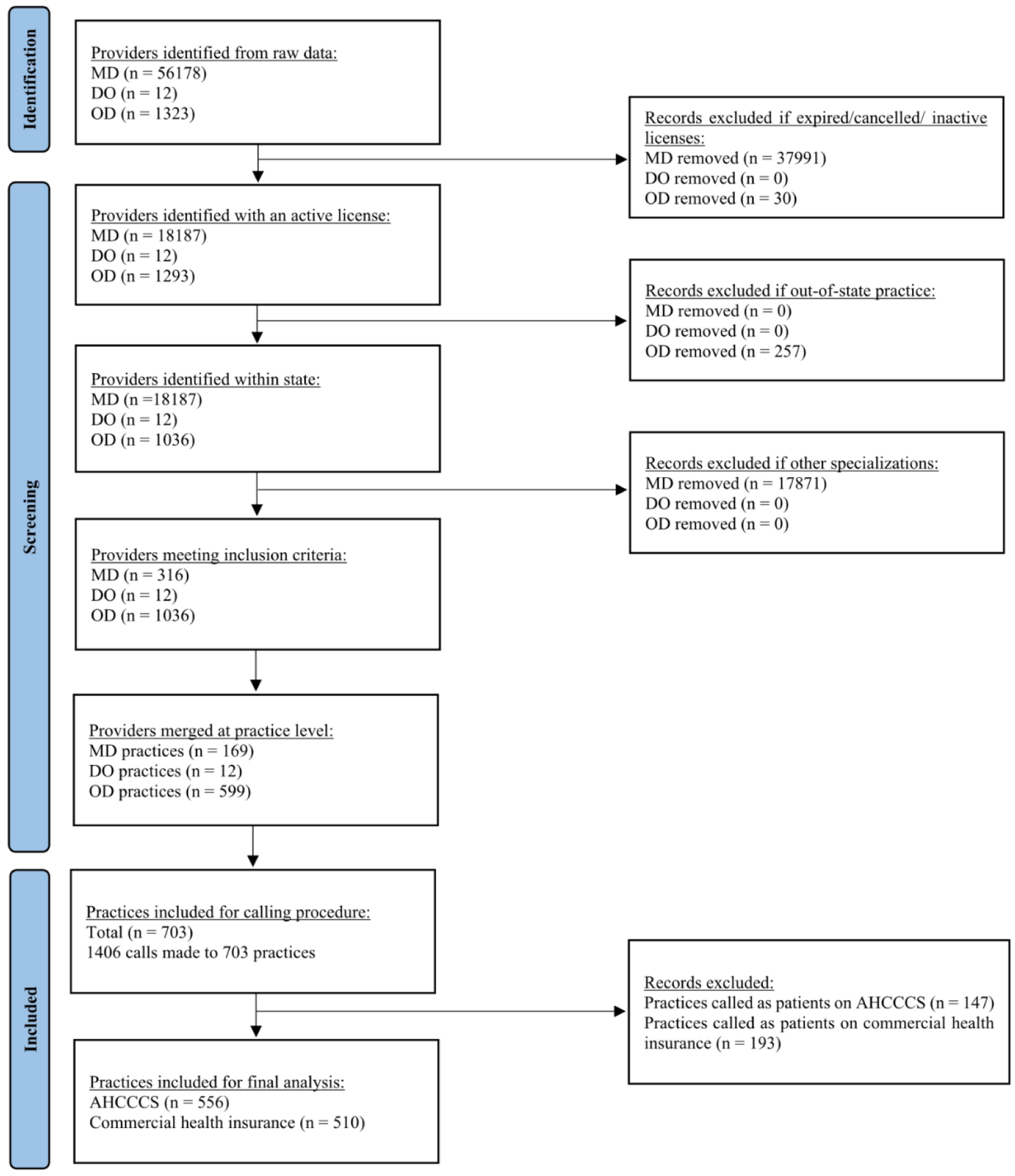
This cross-sectional study assessed the adequacy of pediatric vision care networks in Arizona through a “secret shopper” phone survey. Calls were made to practices that accept Arizona's Medicaid program, Arizona Health Care Cost Containment System (AHCCCS) and/or commercial insurance. Providers were contacted following a standardized script to schedule routine appointments on behalf of 10 and 3-year-old patients enrolled in either Medicaid or commercial health insurance plans. The study examined various components of children's access to vision care services, including the reliability of provider directory information, time until the next available appointment, bilingual service offerings, ages served, region of practice and types of care available.
Results
A total of 556 practices in Arizona were evaluated through simulations as patients on AHCCCS, and 510 practices were assessed through simulations as patients with commercial health insurance plans. The average wait time for the next available appointment was 13 days for both insurance types. Alarmingly, up to 74% of vision care practices in Arizona do not serve children covered by AHCCCS. Furthermore, only 41% provide services to children 5 years and younger.
Conclusions
Our findings underscore the need to improve access to vision care services for children in Arizona, especially racial/ethnic minorities, low-income groups, and rural residents.
- health disparities,
- access to care,
- vision care,
- pediatric,
- network adequacy
Citation: Rizwana Biviji, Nikita Vora, Nalani Thomas, Daniel Sheridan, Cindy M. Reynolds, Faith Kyaruzi, Swapna Reddy. Evaluating the network adequacy of vision care services for children in Arizona: A cross sectional study[J]. AIMS Public Health, 2024, 11(1): 141-159. doi: 10.3934/publichealth.2024007

Related Papers:

Abstract

Background

Vision challenges are among the most prevalent disabling conditions in childhood, affecting up to 28% of school-age children. These issues can impact the development, learning, and literacy skills of affected children. While vision problems are correctable with timely diagnosis and treatment, insufficient networks can impede children's access to comprehensive, and high-quality care.

Objective

The study aims to determine where pediatric vision care network adequacy exists in the state of Arizona and where there are gaps in receiving vision care for children.

Methods

This cross-sectional study assessed the adequacy of pediatric vision care networks in Arizona through a “secret shopper” phone survey. Calls were made to practices that accept Arizona's Medicaid program, Arizona Health Care Cost Containment System (AHCCCS) and/or commercial insurance. Providers were contacted following a standardized script to schedule routine appointments on behalf of 10 and 3-year-old patients enrolled in either Medicaid or commercial health insurance plans. The study examined various components of children's access to vision care services, including the reliability of provider directory information, time until the next available appointment, bilingual service offerings, ages served, region of practice and types of care available.

Results

A total of 556 practices in Arizona were evaluated through simulations as patients on AHCCCS, and 510 practices were assessed through simulations as patients with commercial health insurance plans. The average wait time for the next available appointment was 13 days for both insurance types. Alarmingly, up to 74% of vision care practices in Arizona do not serve children covered by AHCCCS. Furthermore, only 41% provide services to children 5 years and younger.

Conclusions

Our findings underscore the need to improve access to vision care services for children in Arizona, especially racial/ethnic minorities, low-income groups, and rural residents.

Acknowledgments

This project was supported by Virginia G. Piper Charitable Trust, and in partnership with Karen Woodhouse (Director) and Eyes on Learning. Additionally, we would like to extend our heartfelt gratitude and appreciation to the dedicated research assistant Judie Omais for her assistance in the data collection process.

Conflict of interest

There is no conflict of interest in this study.

References

[1]	Centers for Disease Control and PreventionKeep an eye on your vision health (2020). Available from: https://www.cdc.gov/visionhealth/resources/features/keep-eye-on-vision-health.html.
[2]	Medical Optometry AmericaHow often do kids need eye exams? (2021). Available from: https://medodamerica.com/how-often-do-kids-need-eye-exams/
[3]	Gudgel D (2021) Eye screening for children. USA: American Academy of Ophthalmology. Available from: https://www.aao.org/eye-health/tips-prevention/children-eye-screening.
[4]	Ruderman M (2015) Children's Vision and Eye Health: A Snapshot of Current National Issues (1st Ed). The National Center for Children's Vision and Eye Health at Prevent Blindness . Available from: https://preventblindness.org/wp-content/uploads/2016/03/Childrens_Vision_Chartbook_F.pdf.
[5]	Eyes on LearningWhy children's vision matters (2023). Available from: https://eyesonlearning.org/why-childrens-vision-matters/.
[6]	National Center for Children's Vision and Eye Health at Prevent Blindness.Children's Vision and Eye Health: A Snapshot of Current National Issues (2nd Ed.). National Center for Children's Vision and Eye Health at Prevent Blindness (2022) . Available from: https://preventblindness.org/wp-content/uploads/2020/07/Snapshot-Report-2020condensedF.pdf.
[7]	Wittenborn JS, Zhang X, Feagan CW, et al. (2013) The economic burden of vision loss and eye disorders among the United States population younger than 40 years. Ophthalmology 120: 1728-1735. https://doi.org/10.1016/j.ophtha.2013.01.068
[8]	Zambelli-Weiner A, Crews JE, Friedman DS (2012) Disparities in adult vision health in the United States. Am J Ophthalmol 154: S23-S30. https://doi.org/10.1016/j.ajo.2012.03.018
[9]	Ganz M, Xuan Z, Hunter DG (2007) Patterns of eye care use and expenditures among children with diagnosed eye conditions. J AAPOS 11: 480-487. https://doi.org/10.1016/j.jaapos.2007.02.008
[10]	Qiu M, Wang SY, Singh K, et al. (2014) Racial disparities in uncorrected and undercorrected refractive error in the United States. Invest Ophthalmol Vis Sci 55: 6996-7005. https://doi.org/10.1167/iovs.13-12662
[11]	Children's Action AllianceArizona families with children continue to struggle during the pandemic. children's action alliance (2021). Available from: https://azchildren.org/news-and-events/arizona-families-with-children-continue-to-struggle-during-the-pandemic/.
[12]	Arizona Health Care Cost Containment System (AHCCCS)AHCCCS news and press release (2023). Avaialble from: https://www.azahcccs.gov/Shared/News.html.
[13]	AHCCCSAHCCCS members under 21 years of age have eyeglass coverage (2022). Available from: https://www.azahcccs.gov/AHCCCS/Downloads/EyeglassCoverage_2022-2-22.pdf
[14]	Vision screening; administration; rules; notification; definitions. Available from: https://www.azleg.gov/ars/36/00899-10.htm
[15]	Cleveland ClinicEye care specialists (2023). Available from: https://my.clevelandclinic.org/health/articles/8607-eye-care-specialists
[16]	Rankin KA, Mosier-Mills A, Hsiang W, et al. (2022) Secret shopper studies: An unorthodox design that measures inequities in healthcare access. Arch Public Health 80: 226. https://doi.org/10.1186/s13690-022-00979-z
[17]	Haeder SF, Weimer DL, Mukamel DB (2016) Secret shoppers find access to providers and network accuracy lacking for those in marketplace and commercial plans. Health Aff (Millwood) 35: 1160-1166. https://doi.org/10.1377/hlthaff.2015.1554
[18]	Reddy S, Speer M, Saxon M, et al. (2021) Evaluating network adequacy of oral health services for children on Medicaid in Arizona. AIMS Public Health 9: 53-61. https://doi.org/10.3934/publichealth.2022005
[19]	Steinman KJ, Kelleher K, Dembe AE, et al. (2012) The use of a “mystery shopper” methodology to evaluate children's access to psychiatric services. J Behav Health Serv Res 39: 305-313. https://doi.org/10.1007/s11414-012-9275-1
[20]	Steinman KJ, Shoben AB, Dembe AE, et al. (2015) How long do adolescents wait for psychiatry appointments?. Community Ment Health J 51: 782-789. https://doi.org/10.1007/s10597-015-9897-x
[21]	Cama S, Malowney M, Smith AJB, et al. (2017) Availability of outpatient mental health care by pediatricians and child psychiatrists in five US cities. Int J Health Serv 47: 621-635. https://doi.org/10.1177/0020731417707492
[22]	Hsieh HF, Shannon SE (2005) Three approaches to qualitative content analysis. Qual Health Res 15: 1277-1288. https://doi.org/10.1177/1049732305276687
[23]	Cho J, Lee EH (2014) Reducing confusion about grounded theory and qualitative content analysis: Similarities and differences. Qual Rep 19: 1-20. https://doi.org/10.46743/2160-3715/2014.1028
[24]	Kondracki NL, Wellman NS, Amundson DR (2002) Content analysis: Review of methods and their applications in nutrition education. J Nutr Educ Behav 34: 224-230. https://doi.org/10.1016/s1499-4046(06)60097-3
[25]	Biviji R, Williams KS, Vest JR, et al. (2021) Consumer perspectives on maternal and infant health apps: Qualitative content analysis. J Med Internet Res 23: e27403. https://doi.org/10.2196/27403
[26]	Arizona Department of Health ServicesArizona medically underserved areas biennial report (2022). Available from: https://www.azdhs.gov/documents/prevention/health-systems-development/data-reports-maps/reports/azmua-biennial-report.pdf
[27]	AHCCCS 417- Appointment availability, transportation timeliness, monitoring, and reporting. Available from: https://www.azahcccs.gov/shared/Downloads/ACOM/PolicyFiles/400/417_Appointment_Availability_Monitoring_and_Reporting.pdf
[28]	Annual Statistical SupplementMedicaid program description and legislative history (2015). Available from: https://www.ssa.gov/policy/docs/statcomps/supplement/2015/medicaid.html
[29]	Hsiang WR, Lukasiewicz A, Gentry M, et al. (2019) Medicaid patients have greater difficulty scheduling health care appointments compared with private insurance patients: A meta-analysis. Inquiry 56: 46958019838118. https://doi.org/10.1177/0046958019838118
[30]	Wilbur K, Snyder C, Essary AC, et al. (2020) Developing workforce diversity in the health professions: A social justice perspective. Health Prof Educ 6: 222-229. https://doi.org/10.1016/j.hpe.2020.01.002
[31]	Graves JM, Abshire DA, Alejandro AG (2022) System- and individual-level barriers to accessing medical care services across the rural-urban spectrum, Washington State. Health Serv Insights 15: 11786329221104667. https://doi.org/10.1177/11786329221104667
[32]	Anderson NW, Eisenberg D, Zimmerman FJ (2023) Structural racism and well-being among young people in the United States. Am J Prev Med 65: 1078-1091. https://doi.org/10.1016/j.amepre.2023.06.017
[33]	Moss JL, Hearn M, Cuffee YL, et al. (2023) The role of social cohesion in explaining rural/urban differences in healthcare access and health status among older adults in the mid-Atlantic United States. Prev Med 173: 107588. https://doi.org/10.1016/j.ypmed.2023.107588
[34]	HHMGlobal CTThe benefits of online scheduling for healthcare practices (2023). Available from: https://www.hhmglobal.com/knowledge-bank/articles/the-benefits-of-online-scheduling-for-healthcare-practices
[35]	Statistical AtlasThe demographic statistical atlas of the United States (2022). Available from: https://statisticalatlas.com/state/Arizona/Languages
[36]	Jetty A, Jabbarpour Y, Pollack J, et al. (2022) Patient-physician racial concordance associated with improved healthcare use and lower healthcare expenditures in minority populations. J Racial Ethn Disparities 9: 68-81. https://doi.org/10.1007/s40615-020-00930-4/Published
[37]	Sweeney CF, Zinner D, Rust G, et al. (2016) Race/ethnicity and health care communication. Med Care 54: 1005-1009. https://doi.org/10.1097/MLR.0000000000000578
[38]	Ma A, Sanchez A, Ma M (2019) The impact of patient-provider race/ethnicity concordance on provider visits: Updated evidence from the medical expenditure panel survey. J Racial Ethn Health Disparities 6: 1011-1020. https://doi.org/10.1007/s40615-019-00602-y
[39]	Villagra VG, Bhuva B, Coman E, et al. (2019) Health insurance literacy: Disparities by race, ethnicity, and language preference. Am J of Manag Care 25: e71-e75.
[40]	Center For Children and FamiliesMillions of children may lose medicaid: What can be done to help prevent them from becoming uninsured? (2022). Available from: https://ccf.georgetown.edu/2022/02/17/millions-of-children-may-lose-medicaid-what-can-be-done-to-help-prevent-them-from-becoming-uninsured/
[41]	Busch SH, Kyanko KA (2020) Incorrect provider directories associated with out-of-network mental health care and outpatient surprise bills. Health Aff Proj Hope 39: 975-983. https://doi.org/10.1377/hlthaff.2019.01501
[42]	Colvin JD, Hall M, Thurm C, et al. (2018) Hypothetical network adequacy schemes for children fail to ensure patients' access to in-network children's hospital. Health Aff Proj Hope 37: 873-880. https://doi.org/10.1377/hlthaff.2017.1339
[43]	Giovannelli J, Lucia KW, Corlette S (2015) Implementing the affordable care act: State regulation of marketplace plan provider networks. Issue Brief (Commonw Fund) 10: 1-11.
[44]	Hu JC, Cummings JR, Ji X, et al. (2023) Evaluating Medicaid managed care network adequacy standards and associations with specialty care access for children. Health Aff Proj Hope 42: 759-769. https://doi.org/10.1377/hlthaff.2022.01439
[45]	Wong CA, Kan K, Cidav Z, et al. (2017) Pediatric and adult physician networks in affordable care act marketplace plans. Pediatrics 139: e20163117. https://doi.org/10.1542/peds.2016-3117
[46]	Agarwal S Physicians who refuse to accept Medicaid patients breach their contract with society (2017). Available from: https://www.statnews.com/2017/12/28/medicaid-physicians-social-contract/
[47]	Philippe Gwet, Jerrod Anderson, Steven R Out-of-pocket health care expenses in the U.S. civilian noninstitutionalized population by age and insurance coverage, 2014 (2016). Available from: https://meps.ahrq.gov/data_files/publications/st495/stat495.shtml

publichealth-11-01-007-s001.pdf

Reader Comments

Your name:*

Email:*
© 2024 the Author(s), licensee AIMS Press. This is an open access article distributed under the terms of the Creative Commons Attribution License (http://creativecommons.org/licenses/by/4.0)