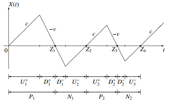
Figure 1.
A sample path of $ X(t) $ with indications of the relevant random variables and the velocities of the motion.


Citation: Terri Rebmann, Kristin D. Wilson, Travis Loux, Ayesha Z. Iqbal, Eleanor B. Peters, Olivia Peavler. Outcomes, Approaches, and Challenges to Developing and Passing a Countywide Mandatory Vaccination Policy: St. Louis County’s Experience with Hepatitis A Vaccine for Food Service Personnel[J]. AIMS Public Health, 2016, 3(1): 116-130. doi: 10.3934/publichealth.2016.1.116
| [1] | Giovanni Scilla, Bianca Stroffolini . Partial regularity for steady double phase fluids. Mathematics in Engineering, 2023, 5(5): 1-47. doi: 10.3934/mine.2023088 |
| [2] | Wenjing Liao, Mauro Maggioni, Stefano Vigogna . Multiscale regression on unknown manifolds. Mathematics in Engineering, 2022, 4(4): 1-25. doi: 10.3934/mine.2022028 |
| [3] | Edgard A. Pimentel, Miguel Walker . Potential estimates for fully nonlinear elliptic equations with bounded ingredients. Mathematics in Engineering, 2023, 5(3): 1-16. doi: 10.3934/mine.2023063 |
| [4] | Aleksandr Dzhugan, Fausto Ferrari . Domain variation solutions for degenerate two phase free boundary problems. Mathematics in Engineering, 2021, 3(6): 1-29. doi: 10.3934/mine.2021043 |
| [5] | Lucio Boccardo, Giuseppa Rita Cirmi . Regularizing effect in some Mingione’s double phase problems with very singular data. Mathematics in Engineering, 2023, 5(3): 1-15. doi: 10.3934/mine.2023069 |
| [6] | Catharine W. K. Lo, José Francisco Rodrigues . On an anisotropic fractional Stefan-type problem with Dirichlet boundary conditions. Mathematics in Engineering, 2023, 5(3): 1-38. doi: 10.3934/mine.2023047 |
| [7] | Menita Carozza, Luca Esposito, Lorenzo Lamberti . Quasiconvex bulk and surface energies with subquadratic growth. Mathematics in Engineering, 2025, 7(3): 228-263. doi: 10.3934/mine.2025011 |
| [8] | Idriss Mazari . Some comparison results and a partial bang-bang property for two-phases problems in balls. Mathematics in Engineering, 2023, 5(1): 1-23. doi: 10.3934/mine.2023010 |
| [9] | Peter Bella, Mathias Schäffner . Local boundedness for $ p $-Laplacian with degenerate coefficients. Mathematics in Engineering, 2023, 5(5): 1-20. doi: 10.3934/mine.2023081 |
| [10] | Giovanni Cupini, Paolo Marcellini, Elvira Mascolo . Local boundedness of weak solutions to elliptic equations with $ p, q- $growth. Mathematics in Engineering, 2023, 5(3): 1-28. doi: 10.3934/mine.2023065 |
Formal models in Neuroscience and Physics are often based on stochastic processes subject to fluctuating behavior due to dichotomous noise. See, for instance, the review given in Bena [1] where some prototypical examples are treated with an emphasis on analytically-solvable cases. An interesting example can be found in Li et al. [2], where a detailed analysis is performed on the effect of correlated dichotomous noises on stochastic resonance in linear systems. See also Jin et al. [3] where a periodic potential driven by multiplicative dichotomous and additive white noise is studied, with special attention to the analysis of coherence resonance and stochastic resonance.
In Theoretical Neuroscience wide interest is devoted to stochastic neuron models driven by dichotomous noise, which constitutes a Markov process that jumps between two states and is characterized by nonvanishing temporal correlations. Recently, various advances have been obtained in this area thanks to the contributions by Müller-Hansen et al. [4] (on the exact derivation of expressions for the probability density and the serial correlation coefficient of the interspike interval in the perfect integrate-and-fire neuron driven by dichotomous noise), by Droste and Lindner [5] (on a thorough analysis of the firing activity of a general integrate-and-fire neuron driven by asymmetric dichotomous noise), and by Mankin and Lumi [6] (on the study of the behavior of a stochastic leaky integrate-and-fire neuron model with temporally correlated input modeled as a colored two-level dichotomous Markovian noise).
A landmark among stochastic processes driven by dichotomous noise is the (integrated) telegraph process. It is also known as Goldstein-Kac telegraph process after Goldstein [7] and Kac [8]. These initial contributions were finalized to construct a stochastic model for the motion of a particle that runs on the real line with constant speed and alternates between two possible directions of motion at random homogeneous Poisson-paced time instants (see Kolesnik and Ratanov [9], and references therein). Typical approaches to the determination of the probability distribution of the telegraph process are analytical or based on transformations (see, e.g. Orsingher [10], Beghin et al. [11], López and Ratanov [12]). Among the various generalizations proposed in the recent literature we recall the alternating motion with random delays (cf. Bshouty et al. [13]), and the alternating damped motion studied by Di Crescenzo and Martinucci [14], and De Gregorio and Macci [15]. Other recent investigations have been devoted to suitable functionals of telegraph processes (cf. Kolesnik [16] and [17], Martinucci and Meoli [18]), to dynamics in the presence of an elastic boundary (see Di Crescenzo et al. [19]), and to level-crossings problems (cf. Pogorui et al. [20]). Moreover, applications of telegraph processes are found to be useful in the area of financial mathematics, especially when jumps are allowed at the switching instants (cf. Ratanov [21], for instance). Further studies have been oriented to modeling random phenomena by means of Brownian motion with drift following the telegraph process (see Di Crescenzo and Zacks [22] for a case of interest in environmental sciences, and Travaglino et al. [23] for an application in mathematical geosciences). Recent developments show that a multi-dimensional version of the telegraph process can be used to construct new efficient and flexible families of Monte Carlo methods (see Bierkens et al. [24]).
The analysis of the telegraph process and its modifications often involves hyperbolic equations with constant coefficients. More general instances concerning parameters varying in space and time are more difficult to be treated. A first contribution in this field is a case of time-dependent rates (cf. Iacus [25]). Recent advances on state-dependent generalizations of the telegraph process have been provided by Garra and Orsingher [26]. Nevertheless, state-dependent stochastic processes deserve interest in neuronal modeling, as for diffusion neuronal models with multiplicative noise (D'Onofrio et al. [27]) and for processes with exponential decay subject to excitatory inputs with state-dependent effects (Di Crescenzo and Martinucci [28]).
Stimulated by the above investigations, hereafter we analyze a modified telegraph process describing fluctuating behavior with variable trend, where the fluctuations follow a state-dependent alternation. Specifically, we consider a state-dependent telegraph process with constant opposite velocities, and with switching intensities that vanish when the motion is directed toward the zero state. In other terms, if the motion has positive (negative) velocity, then the switch to negative (positive) velocity may occur -depending on the state- only if the state is positive (negative). This ensures that consecutive velocity changes are separated by passages through the zero state. The resulting motion is thus describing particles that move with alternating constant velocities and fluctuate around the origin. Clearly, the considered random motion is governed by the hazard rates of the interarrival times between consecutive velocity changes. When the hazard rates are not constant, obtaining the solutions of the resulting partial differential equations for the transition densities becomes difficult. However in our case, in which the hazard rates depend on both the position and the velocity of the motion, we adopt a different approach. This is based on renewal theory which has turned out to be useful in some instances considered in the past (see, e.g., Di Crescenzo [29] for the case of Erlang-distributed random times separating velocity reversals). The renewal-based approach allows us to determine the formal expressions of the probability density functions of the motion during suitable time intervals. We also investigate a special case, in which the interarrival times are related to the gamma distribution so that the probability density functions can be expressed in closed form. A first-passage-time problem is also treated when the process is constrained between two boundaries, with an analysis based on a suitable index taking values in $ [0, 1] $, and defined as a ratio of mean values.
It is worth mentioning that the results obtained in this paper can be used in various applied fields, especially in Biomathematics. Indeed, stochastic processes describing finite-velocity random motions constitute a valide alternative to diffusion processes since the latter processes exhibit certain features, such as the unboundedness of the first variation, that are not appropriate to describe real phenomena. For instance, various stochastic models based on telegraph equations, such as persistent random walks, are finalized to describe appropriate population dynamics or individual animal movement (for instance, cf. Alharbi and Petrovskii [30], Angelani and Garra [31], Garcia et al. [32]).
This is the plan of the paper. In Section 2 we describe in detail the state-dependent telegraph process. We also introduce the forward and backward transition densities of the motion, and the random variables describing the time intervals during which the motion is forward or backward. Section 3 is centered on the determination of the formal expressions of the transition densities of the process. In Section 4 we deal with a special case when the interarrival times have gamma distribution. This instance corresponds to suitable monotonic intensity functions which allow to obtain the transition densities of the motion in closed form, expressed in terms of the generalized (two-parameter) Mittag-Leffler function. Section 5 is concerning a first-passage-time problem for the considered process in the presence of two boundaries. Finally, some concluding remarks are given in Section 6.
We consider a state-dependent telegraph process $ \{X(t), t\geq 0\} $, which describes the alternating behavior of a suitable stochastic system, such as the motion of a particle running on the real line. The particle velocity, say $ V(t) $, alternates randomly between the fixed values $ c > 0 $ and $ -v < 0 $. We assume that the initial position is $ X(0) = 0 $ and the initial velocity is $ V(0) = c $.
Let $ f(x, t) $ and $ b(x, t) $ denote respectively the forward and backward transition densities of the motion, defined as
| $ f(x,t):=∂∂xP{X(t)≤x,V(t)=c},b(x,t):=∂∂xP{X(t)≤x,V(t)=−v}. $ | (2.1) |
For $ t > 0 $ and $ -vt < x < ct $, densities (2.1) satisfy the following partial differential equations:
| $ \left\{∂∂tf(x,t)+c∂∂xf(x,t)=−λ+(x)f(x,t)+λ−(x)b(x,t),∂∂tb(x,t)−v∂∂xb(x,t)=−λ−(x)b(x,t)+λ+(x)f(x,t),\right.$ | (2.2) |
where $ \lambda^+(x) $ and $ \lambda^-(x) $ are nonnegative functions, for all $ x\in \mathbb R $. The function $ \lambda^+(x) $ represents the intensity of velocity changes when the particle occupies state $ x $ with current forward motion, and similarly $ \lambda^-(x) $ represents the same intensity for the backward motion. Clearly, for the classical telegraph process the intensity functions $ \lambda^+(x) $ and $ \lambda^-(x) $ are constant, leading to exponentially distributed interarrival times between consecutive velocity changes. Instead, herein we assume that they depend on the position $ x $ and satisfy the following assumptions:
| $\left\{λ+(x)=0 if x≤0,λ−(x)=0 if x≥0,\right. $ | (2.3) |
and
| $ ∫+∞0λ±(±x)dx=+∞. $ | (2.4) |
The conditions (2.3) express that each instant a velocity change occurs, then the process is forced to return to the 0 state prior to the subsequent velocity change (see the sample path of $ X(t) $ shown in Figure 1). Specifically, changes from positive to negative velocity occur only if the particle occupies a positive state $ x $, whereas the opposite velocity changes occur only at negative states. The assumption (2.4) provide a bona fide condition, whose role will be clarified in the following. Clearly, the given assumptions imply that consecutive velocity changes of the motion are separated by passages through the zero state. The resulting state-dependent telegraph process is then useful to describe systems that alternate randomly around the 0 level.
We remark that other stochastic processes describing alternating motions governed by non-constant parameters have been treated recently by Garra and Orsingher [26]. Specifically, some cases of space-varying velocities and time-varying intensity are treated by means of suitable space-time transformations.
We point out that performing a transformation analogous to Eq. (2.3) of Beghin et al. [11], the equations (2.2) lead to a system of partial differential equations for the transition density $ p(x, t) $ and the flow function $ w(x, t) $ of the process $ X(t) $, defined respectively as
| $ p(x,t):=∂∂xP{X(t)≤x}=f(x,t)+b(x,t),w(x,t):=f(x,t)−b(x,t). $ | (2.5) |
According to Orsingher [10], in a large ensemble of particles moving as specified, the function $ w(x, t) $ can be viewed as a measure of the excess of particles moving forward with respect to those moving backward near point $ x $ at time $ t $.
In this section we analyze the probabilistic structure of the random variables that describe the upward and downward particle motion.
For every $ i\in \mathbb N $, we denote by $ U_i $ (respectively $ D_i $) the random duration of the $ i $-th time interval in which the motion has positive (negative) velocity. For any $ i\in \mathbb N $, we express $ U_i $ as the sum of the random time length $ U_i^- $ during which $ X(t) < 0 $, and the random time length $ U_i^+ $ during which $ X(t) > 0 $. Clearly, since the initial velocity is positive, one has
| $ U_1^- = 0\quad \hbox{and} \quad U_1 = U_1^+. $ |
Similarly we have (see Figure 1)
| $ D_i = D_i^++D_i^-, \qquad i\in \mathbb N. $ |
From the assumptions (2.3) and (2.4) it follows that the passages of $ X(t) $ through the 0 state are regenerative alternating events, and the dynamics of the velocity changes do not depend on time. Hence, the sequence $ \{U_i^+; i\in \mathbb N\} $ is formed by independent and identically distributed random variables. The same conclusion holds for the independent sequence $ \{D_i^-; i\in \mathbb N\} $.
We denote with $ Z_i $ the $ i $-th random instant in which the process is equal to 0, and with $ P_i $ (resp. $ N_i $) the duration of the $ i $-th time interval in which $ X(t) $ is positive (negative), as shown in Figure 1. It is easy to verify that, for every $ i\in\mathbb N $,
| $\left\{Pi=Z2i−1−Z2(i−1),Ni=Z2i−Z2i−1,\right.$ | (2.6) |
where $ Z_0: = 0 $. From the assumptions on the motion, the following relationships are straightforward (as shown in Figure 1)
| $ cU_i^+-vD_i^+ = 0, \qquad -vD_i^-+cU_{i+1}^- = 0, $ |
so that
| $ \left\{Pi=U+i+D+i=c+vvU+i,Ni=D−i+U−i+1=c+vcD−i,\right.$ | (2.7) |
Thus, the sequences $ \{P_i; i\in \mathbb N\} $ and $ \{N_i; i\in \mathbb N\} $ are independent and, clearly, they are formed by independent and identically distributed random variables.
Since the motion proceeds with constant velocities, and the instants $ \{Z_{2i}; i\in \mathbb N\} $ and $ \{Z_{2i-1}; i\in \mathbb N\} $ are regenerative, a linear time-transformation allows the functions $ \lambda^+(x) $ and $ \lambda^-(x) $ in Eqs. (2.2) to represent the intensities of occurrence of velocity changes along the time axes. Hence, from classical arguments of renewal theory, it follows that $ \lambda^+(x) $ and $ \lambda^-(-x) $, for $ x\geq 0 $, are respectively the hazard rate functions of $ c U_i^+ $ and $ v D_i^- $ at $ x\geq 0 $, i.e.
| $ \lambda^+(x) = \lim\limits_{h\to 0^+}\frac{1}{h} {\mathbb P}\{c U_i^+\leq x+h \,|\, c U_i^+ \gt x\}, $ |
| $ \lambda^-(-x) = \lim\limits_{h\to 0^+}\frac{1}{h} {\mathbb P}\{v D_i^-\leq x+h \,|\, v D_i^- \gt x\}. $ |
Here and throughout the paper, we denote by $ \overline{F}_Y(x) = {\mathbb P}\{Y > x\} $ the complementary distribution function of a random variable $ Y $. We can thus introduce the following expressions, for $ x\geq 0 $,
| $ ¯FcU+i(x)=exp{−∫x0λ+(y)dy}=e−Λ+(x),¯FvD−i(x)=exp{−∫x0λ−(−y)dy}=e−Λ−(x), $ | (2.8) |
where
| $ Λ±(x):=∫x0λ±(±y)dy,x≥0, $ | (2.9) |
constitute the corresponding cumulative hazard rates. Hence, we immediately obtain the probability density functions of $ U_i^+ $ and $ D_i^- $, namely
| $ f_{U_i^+}(x) = c\lambda^+(cx)e^{-\Lambda^+(cx)}, \qquad f_{D_i^-}(x) = v\lambda^-(-vx)e^{-\Lambda^-(vx)}, \qquad x \gt 0. $ |
Consequently, the random variables $ U_i^+ $ and $ D_i^- $ are nonnegative, absolutely continuous, for all $ i\in \mathbb N $, with distribution functions
| $ FU+i(x)=1−e−Λ+(cx),FD−i(x)=1−e−Λ−(vx),x>0, $ | (2.10) |
respectively. Moreover, due to assumption (2.4), they are honest random variables, in the sense that they take values over $ \mathbb{R} $ with probability 1. Finally, the relations (2.7) permit us to express the complementary distribution functions of $ P_i $ and $ N_i $, $ i\in \mathbb N $, as follows, for $ x\geq 0 $,
| $ \overline{F}_{P_i}(x) = \exp\bigg\{ -\Lambda^+\Big( \frac{cv}{c+v}x \Big) \bigg\}, \qquad \overline{F}_{N_i}(x) = \exp\bigg\{ -\Lambda^-\Big( \frac{cv}{c+v}x \Big) \bigg\}. $ |
On the ground of the above results, we are now able to express the dependence of the process $ X(t) $ on the regenerative random times $ Z_i $. Indeed, if $ k $ velocity changes occurred in $ [0, t] $, $ t > 0 $, then
| $ X(t)=Vk(t−Zk), $ | (2.11) |
where
| $ V_k = \left\{ c,k even−v,k odd. \right. $ |
Consequently, the process $ X(t) $ can be expressed as
| $ X(t) = \sum\limits_{k = 0}^{\infty} \mathbb{1}_{\{C(t) = k\}} V_k\,(t-Z_k), \qquad t \gt 0, $ |
where $ \mathbb{1}_{A} $ is the indicator function of $ A $, i.e. $ \mathbb{1}_{A} = 1 $ if $ A $ is true, and $ \mathbb{1}_{A} = 0 $ otherwise, and where $ C(t) $ is the alternating counting process that counts the number of velocity changes in $ [0, t] $, whose interarrival times are $ U_1, D_1, U_2, D_2, \ldots $
In this section we determine the formal expressions of the probability density functions that describe the motion during suitable time intervals. Specifically, with reference to the random variables introduced in Section 2.1, we deal with the following densities, for $ n\in\mathbb N $,
| $ fn(x,t):=∂∂xP{X(t)≤x,Z2(n−1)−U−n≤t<Z2(n−1)+U+n},bn(x,t):=∂∂xP{X(t)≤x,Z2n−1−D+n≤t<Z2n−1+D−n}. $ | (3.1) |
Clearly, for each $ n\in\mathbb N $, $ f_n(x, t) $ (resp. $ b_n(x, t) $) represents the forward (backward) density of the particle position at time $ t $, during the $ n $-th period in which the motion has positive (negative) velocity. Hence, the densities defined in (2.1) can be expressed by
| $ f(x,t)=∞∑n=1fn(x,t),b(x,t)=∞∑n=1bn(x,t), $ | (3.2) |
provided that the above series are convergent. Before determining the forward densities given in the first of (3.1) we recall that, since the initial velocity is positive, the state space of the particle position at time $ t $ is $ (-vt, ct] $, and the probability law of $ X(t) $ has a discrete component at point $ ct $, so that the density $ f_1(x, t) $ is degenerate.
Theorem 3.1. The forward probability densities defined in the first of (3.1) can be expressed as follows:
| $ f1(x,t)=¯FU+1(t)δ(ct−x),x∈R,t≥0, $ | (3.3) |
where $ \delta(x) $ denotes the Dirac delta function, and, for $ n = 2, 3, \dots $,
| $ fn(x,t)={1cfZ2(n−1)(t−xc)¯FU+n(xc),0<x<ct,1c+v∫t+xv0fD−n−1(c(t−z)−xc+v)fZ2n−3(z)dz,−vt<x<0. $ | (3.4) |
Proof. If $ t < U_1^+ $, then no changes of velocity have occurred up to time $ t $, and so $ X(t) = ct $. Thus, equation (3.3) follows immediately since the relevant distribution has an atom at the point $ x = ct $. Note that the density $ f_1(x, t) $ must be intended as a generalized function. It is clear that in the $ n $-th period in which the velocity is positive $ X(t) = c(t-Z_{2(n-1)}) $, as stated in equation (2.11) for $ k = 2n-1 $, and confirmed by Figure 1. So that, for $ n > 1 $ and $ 0 < x < ct $ we have
| $ P{X(t)≤x,Z2(n−1)<t<Z2(n−1)+U+n}=P{c(t−Z2(n−1))≤x,U+n>t−Z2(n−1),Z2(n−1)<t}=∫t0P{c(t−Z2(n−1))≤x,U+n>t−Z2(n−1)|Z2(n−1)=z}P{Z2(n−1)∈dz}=∫t0P{c(t−z)≤x,U+n>t−z}P{Z2(n−1)∈dz}=∫tt−xc¯FU+n(t−z)fZ2(n−1)(z)dz. $ | (3.5) |
Differentiating with respect to $ x $ we thus obtain the density (3.4) for $ 0 < x < ct $. Furthermore, for $ n = 2, 3, \dots $ and $ -vt < x < 0 $, in the $ n $-th period in which the velocity is positive one has
| $ X(t)=−vD−n−1+c(t−Z2n−3−D−n−1)=ct−cZ2n−3−(c+v)D−n−1. $ |
So that, similarly to (3.5), we have
| $ P{X(t)≤x,Z2(n−1)−U−n≤t<Z2(n−1)}=P{X(t)≤x,Z2n−3+D−n−1≤t<Z2n−3+c+vcD−n−1}=P{ct−cZ2n−3−(c+v)D−n−1≤x,D−n−1≤t−Z2n−3<c+vcD−n−1}=∫t0P{c(t−z)−(c+v)D−n−1≤x,D−n−1≤t−z<c+vcD−n−1}P{Z2n−3∈dz}=∫t0P{D−n−1≥c(t−z)−xc+v,D−n−1>c(t−z)c+v,D−n−1≤t−z}P{Z2n−3∈dz}=∫t0P{D−n−1≥c(t−z)−xc+v,D−n−1≤t−z}P{Z2n−3∈dz}=∫t01{c(t−z)−xc+v≤t−z}P{c(t−z)−xc+v≤D−n−1≤t−z}P{Z2n−3∈dz}=∫t+xv0[FD−n−1(t−z)−FD−n−1(c(t−z)−xc+v)]fZ2n−3(z)dz. $ |
Differentiating with respect to $ x $ we finally get the density (3.4) for $ -vt < x < 0 $.
A similar result can be obtained for the densities introduced in the second line of (3.1).
Theorem 3.2. For $ n\in \mathbb{N} $, the backward probability densities defined in the second of (3.1) can be expressed as
| $ bn(x,t)={1vfZ2n−1(t+xv)¯FD−n(−xv),−vt<x<0,1c+v∫t−xc0fU+n(x+v(t−z)c+v)fZ2(n−1)(z)dz,0<x<ct. $ | (3.6) |
Proof. The proof is omitted, being very similar to that of the previous theorem.
Let us define the '$ n $-th cycle' as the random interval formed by the $ n $-th period when the particle has positive velocity and the $ n $-th period when the particle has negative velocity. Clearly,
| $ pn(x,t):=∂∂xP{X(t)≤x,Z2(n−1)−U−n≤t<Z2n−1+D−n} $ | (3.7) |
is the density of the particle position at time $ t $ during the $ n $-th cycle. Due to (3.1), the density (3.7) can be easily obtained from Theorem 3.1 and Theorem 3.2, being
| $ p_n(x,t) = f_n(x,t)+b_n(x,t). $ |
As a consequence, the transition density introduced in the first of (2.5) can be also expressed as
| $ p(x,t) = \sum\limits_{n = 1}^{\infty}p_n(x,t), $ |
provided that the above series is convergent.
The aim of this section is to analyze in detail the case in which the upward and downward displacements performed by the particle after passages though the zero state have gamma distribution. Specifically, we assume that the random variables $ cU_i^+ $ and $ vD_i^- $, $ i\in \mathbb{N} $, are gamma distributed with shape parameters $ \alpha $ and $ \alpha^* $, respectively, and equal rate parameters $ \beta $, say
| $ cU+i∼Gamma(α,β),vD−i∼Gamma(α∗,β), $ | (4.1) |
where $ \alpha, \alpha^*, \beta > 0 $. We recall that the telegraph process with gamma-distributed intertimes between velocity changes has been analyzed in Di Crescenzo and Martinucci [33], whereas some suitable multidimensional random motions with step lengths having gamma distribution have been investigated in Le Caër [34] and Pogorui and Rodríguez-Dagnino [35], for instance.
Clearly, the assumptions (4.1) correspond to the case in which the intensity functions $ \lambda^+(x) $ and $ \lambda^-(x) $ are given by
| $ λ+(x)=βαxα−1e−βxΓ(α,βx),λ−(−x)=βα∗xα∗−1e−βxΓ(α∗,βx),x>0, $ | (4.2) |
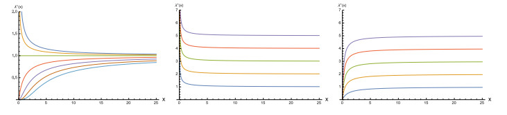
where $ \Gamma(\cdot, \cdot) $ denotes the upper incomplete gamma function. We remark that such intensity functions are strictly decreasing (increasing) in $ |x| $ if $ 0 < \alpha < 1 $ ($ \alpha > 1 $), and are constant if $ \alpha = 1 $, with
| $ \lim\limits_{x\to 0^+}\lambda^+(x) = \left\{ +∞,0<α<1,β,α=1,0,α>1, \right. \qquad \lim\limits_{x\to +\infty}\lambda^{+}(x) = \beta, $ |
with analogous limits holding for $ \lambda^-(x) $. See Figure 2 for some plots of $ \lambda^+(x) $. We remark that, from the assumptions given in (4.1), one also has
| $ U+i∼Gamma(α,cβ),D−i∼Gamma(α∗,vβ). $ | (4.3) |
In the following theorems we obtain the forward and backward transition densities (2.1) in a special case. Such densities will be expressed in terms of the generalized (two-parameter) Mittag-Leffler function, defined as
| $ Ea,b(z):=∞∑n=0znΓ(an+b). $ | (4.4) |
Properties and results on such Mittag-Leffler function can be found, for instance, in Gorenflo et al. [36], Haubold et al. [37] and references therein. We recall that function (4.4) has been used recently in the analysis of probability distributions of some birth-death type processes in Alipour et al. [38], Di Crescenzo et al. [39] and Orsingher and Polito [40].
Theorem 4.1. Let $ \{X(t), t\geq 0\} $ be the state-dependent telegraph process with intensity functions specified in (4.2). For $ t > 0 $, the forward transition density is given by
| $ f(x,t)=Γ(α,βct)Γ(α)δ(ct−x)+Γ(α,βx)Γ(α)1ct−x((ct−x)vβc+v)α+α∗×exp{−(ct−x)vβc+v}Eα+α∗,α+α∗(((ct−x)vβc+v)α+α∗)1{x<ct},0<x≤ct, $ | (4.5) |
| $ f(x,t)=cαΓ(α∗)(vβc+v)α+α∗exp{−vβ(ct−x)c+v}×∫t+xv0(c(t−z)−x)α∗−1zα−1Eα+α∗,α((cvβzc+v)α+α∗)dz,−vt<x<0. $ | (4.6) |
Proof. From (3.2), (3.3), the first case of (3.4) and (4.3) we easily obtain, for $ 0 < x\leq ct $,
| $ f(x,t)=Γ(α,βct)Γ(α)δ(ct−x)+Γ(α,βx)Γ(α)1c∞∑n=2fZ2(n−1)(t−xc). $ | (4.7) |
In order to analyze the distribution of $ Z_{2(n-1)} $ we note that, from the relationships (2.7), one has
| $ P_i\sim {\rm Gamma}\bigg(\alpha, \frac{cv}{c+v}\beta\bigg), \qquad N_i\sim {\rm Gamma}\bigg(\alpha^*, \frac{cv}{c+v}\beta \bigg), $ |
and thus
| $ n∑i=1Pi∼Gamma(nα,cvc+vβ),n∑i=1Ni∼Gamma(nα∗,cvc+vβ). $ | (4.8) |
We point out that, due to (2.6), for the regenerative random times $ Z_{i} $ one has
| $ Z_{2n} = \sum\limits_{i = 1}^{n} (P_i+N_i), \qquad Z_{2n-1} = Z_{2(n-1)}+P_n, \qquad n\in \mathbb N. $ |
Hence, since the gamma-distributed random variables in (4.8) have identical rates, we get
| $ Z2n∼Gamma(n(α+α∗),cvc+vβ),Z2n−1∼Gamma((n−1)(α+α∗)+α,cvc+vβ). $ |
Such relations, thanks to (4.4), allow to compute the following sum:
| $ 1c∞∑n=2fZ2(n−1)(t−xc)=1cexp{−(ct−x)vβc+v}∞∑n=2(cvβc+v)(n−2)(α+α∗)+(α+α∗)Γ((n−2)(α+α∗)+(α+α∗))(t−xc)(n−2)(α+α∗)+(α+α∗)−1=1ct−xexp{−(ct−x)vβc+v}((ct−x)vβc+v)α+α∗∞∑n=0(((ct−x)vβc+v)α+α∗)nΓ(n(α+α∗)+(α+α∗))=1ct−xexp{−(ct−x)vβc+v}((ct−x)vβc+v)α+α∗Eα+α∗,α+α∗(((ct−x)vβc+v)α+α∗). $ | (4.9) |
Substituting (4.9) in (4.7) we finally obtain (4.5). Similarly, from (3.2) and the second of (3.4) we obtain, for $ -vt < x < 0 $,
| $ f(x,t)=1c+v∫t+xv0∞∑n=2fD−n−1(c(t−z)−xc+v)fZ2n−3(z)dz=1c+v∫t+xv0fD−1(c(t−z)−xc+v)∞∑n=0fZ2n+1(z)dz=1c+v(vβ)α∗Γ(α∗)∫t+xv0(c(t−z)−xc+v)α∗−1exp{−vβ(c(t−z)−x)c+v}×exp{−cvβzc+v}∞∑n=0(cvβc+v)n(α+α∗)+αΓ(n(α+α∗)+α)zn(α+α∗)+α−1dz=1Γ(α∗)(vβc+v)α∗exp{−vβ(ct−x)c+v}×∫t+xv0(c(t−z)−x)α∗−1(cvβzc+v)α1z∞∑n=0((cvβzc+v)α+α∗)nΓ(n(α+α∗)+α)dz=cαΓ(α∗)(vβc+v)α+α∗exp{−vβ(ct−x)c+v}×∫t+xv0(c(t−z)−x)α∗−1zα−1Eα+α∗,α((cvβzc+v)α+α∗)dz, $ | (4.10) |
which finally gives Eq. (4.6).
The following theorem is a companion of Theorem 4.1.
Theorem 4.2. Let $ \{X(t), t\geq 0\} $ be the state-dependent telegraph process with intensity functions specified in (4.2). For $ t > 0 $, the backward transition density is:
| $ b(x,t)=Γ(α∗,−βx)Γ(α∗)1vt+x(c(vt+x)βc+v)α×exp{−c(vt+x)βc+v}Eα+α∗,α((c(vt+x)βc+v)α+α∗),−vt<x<0, $ | (4.11) |
| $ b(x,t)=vα+α∗Γ(α)(cβc+v)2α+α∗exp{−cβ(x+vt)c+v}×∫t−xc0(x+v(t−z))α−1zα+α∗−1Eα+α∗,α+α∗((cvβzc+v)α+α∗)dz,0<x<ct. $ | (4.12) |
Proof. The proof is omitted, being similar to that of Theorem 4.1.
Combining the results of the previous theorems with relationships (2.5) one can easily calculate the transition density and the flow function of the process $ X(t) $.
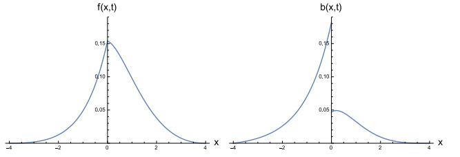
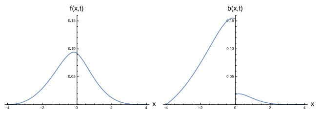
As example, in Figure 3 and 4 we show some plots of the (absolutely continuous component) of densities $ f(x, t) $ and $ b(x, t) $.
Unfortunately, obtaining approximate results from Theorems 4.1 and 4.2 by means of asymptotic expansions of the Mittag-Leffler function seems to be not fruitful, since the available expressions are quite cumbersome (see, for instance, Haubold et al. [37]).
If $ \alpha = \alpha^* = 1 $, then the intensity rates (4.2) are constants and thus the corresponding cumulative hazard rates (2.9) are linear in $ x $, i.e. the random times $ U_i^+ $ and $ D_i^- $ are exponentially distributed. This special case leads to simpler closed-form results, as shown hereafter.
Corollary 4.1. Let $ \{X(t), t\geq 0\} $ be the state-dependent telegraph process with intensity functions $ \lambda^+(x) = \lambda^-(-x) = \beta $, $ x > 0 $. For $ t > 0 $, the forward and backward transition density are:
| $ f(x,t)={e−βctδ(ct−x)+12e−βxvβc+v(1−exp{−2(ct−x)vβc+v})1{x<ct},0<x≤ct,12eβxvβc+v(1−exp{−2c(vt+x)βc+v}),−vt<x<0, $ | (4.13) |
| $ b(x,t)={12e−βxcβc+v(1−exp{−(ct−x)vβc+v})2,0<x<ct,12eβxcβc+v(1+exp{−2c(vt+x)βc+v}),−vt<x<0. $ | (4.14) |
Proof. The proof follows from Theorems 4.1 and 4.2 after some calculations, and noting that $ E_{2, 1}(z) = \cosh(\sqrt{z}) $ and $ E_{2, 2}(z) = \sinh(\sqrt{z})/\sqrt(z) $.
We remark that the results obtained so far are concerning the case with positive initial velocity, i.e. $ V(0) = c $. However, the case $ V(0) = -v $ can be treated in a similar way, by exploting suitable symmetries. Specifically, the probability law of $ X(t) $ conditional on $ V(0) = -v $ can be obtained from the above results by interchanging the forward density with the backward one, the distribution of $ U_i^{\pm} $ with that of $ D_i^{\mp} $, $ c $ with $ v $, and $ x $ with $ -x $. Clearly, this allows us to analyze more general situations, in which the initial velocity is random, i.e. $ {\mathbb P}\{V(0) = c\} = \theta $ and $ {\mathbb P}\{V(0) = -v\} = 1-\theta $, $ 0\leq \theta\leq 1 $, when the distributions of interest are expressed as suitable mixtures.
This section is devoted to a first-passage-time problem for the process $ X(t) $, assuming the presence of two boundaries, say $ \eta > 0 $ and $ -\xi < 0 $. Hereafter we thoroughly assume that, in addition to assumptions (2.3) and (2.4), the intensity functions $ \lambda^+(x) $ and $ \lambda^-(x) $ satisfy the following condition:
| $ ∫t0λ±(±x)dx<+∞for any t>0. $ | (5.1) |
With reference with the notions introduced in Section 2.1, we denote by
| $ M^+(t) = \sum\limits_{n = 0}^{\infty} \mathbb{1}_{\{Z_{2n}\leq t\}} $ |
the right-continuous counting process whose increments occur at the random instants $ 0 = Z_0, Z_2, Z_4, \ldots $, so that
| $ M^+(Z_{2n}) = n+1, \qquad n \in \mathbb{N}_0. $ |
We denote by
| $ T_{\zeta} = \inf\{t \gt 0: X(t) = \zeta\}, \qquad \zeta \neq 0 $ |
the first-passage time of $ X(t) $ through the boundary $ \zeta \neq 0 $. Then we introduce the integer-valued random variable $ M^+(T_{\eta}) $. Recalling that the $ i $-th time interval in which the motion has positive velocity (upward period, say) has random duration $ U_i $, $ i\in \mathbb N $, let $ M^+(T_{\eta}) $ denote the ordinal number of the first of such upward periods in which $ X(t) $ crosses the boundary $ \eta > 0 $. Clearly, due to the first of (2.10) we have
| $ P{M+(Tη)=k}=P{cU+1<η,…,cU+k−1<η,cU+k≥η}=k−1∏i=1FU+i(ηc)¯FU+k(ηc)=(1−e−Λ+(η))k−1e−Λ+(η),k∈N. $ | (5.2) |
Hence, $ M^+(T_{\eta}) $ has geometric distribution with parameter $ e^{-\Lambda^+(\eta)} $, where $ \Lambda^+(x) $ is defined in (2.9). It thus follows that
| $ E[M+(Tη)]=eΛ+(η). $ | (5.3) |
Similarly,
| $ M^-(t) = \sum\limits_{n = 0}^{\infty} \mathbb{1}_{\{Z_{2n+1}\leq t\}} $ |
is the right-continuous counting process whose increments occur at the random instants $ Z_1, Z_3, Z_5, \ldots $, and thus
| $ M^-(Z_{2n+1}) = n+1, \qquad n \in \mathbb{N}_0. $ |
For $ \xi > 0 $, we can thus introduce the integer-valued random variable $ M^-(T_{-\xi}) $. In analogy with $ M^+(T_{\eta}) $, we assume that $ M^-(T_{-\xi}) $ gives the ordinal number of the first downward period in which $ X(t) $ crosses the boundary $ -\xi < 0 $. Similarly as in (5.2), $ M^-(T_{-\xi}) $ has geometric distribution with parameter $ e^{-\Lambda^-(\xi)} $, so that its expectation is
| $ E[M−(T−ξ)]=eΛ−(ξ). $ | (5.4) |
Let us now consider the first-passage-time problem in the presence of two boundaries. We consider the random variable
| $ M(−ξ,η):=min{M+(Tη),M−(T−ξ)}. $ | (5.5) |
Since, for $ k\in \mathbb N $,
| $ P{M(−ξ,η)=k}=P{cU+1<η,vD−1<ξ,…,cU+k−1<η,vD−k−1<ξ,cU+k≥η}+P{cU+1<η,vD−1<ξ,…,cU+k−1<η,vD−k−1<ξ,cU+k<η,vD−k≥ξ}=(1−e−Λ+(η))k−1(1−e−Λ−(ξ))k−1{e−Λ+(η)+(1−e−Λ+(η))e−Λ−(ξ)}=(1−e−Λ+(η)−e−Λ−(ξ)+e−Λ+(η)e−Λ−(ξ))k−1{e−Λ+(η)+e−Λ−(ξ)−e−Λ+(η)e−Λ−(ξ)}, $ |
it follows that $ M(-\xi, \eta) $ has geometric distribution with parameter $ e^{-\Lambda^+(\eta)}+e^{-\Lambda^-(\xi)}-e^{-\Lambda^+(\eta)}e^{-\Lambda^-(\xi)} $ and expectation
| $ E[M(−ξ,η)]=1e−Λ+(η)+e−Λ−(ξ)−e−Λ+(η)e−Λ−(ξ). $ | (5.6) |
We remark that the assumption (5.1) ensures that the expectations given in (5.3), (5.4) and (5.6) are finite.
Let us now consider the special case of interarrival times having gamma distribution like in Section 4.
Proposition 5.1. Let $ \{X(t), t\geq 0\} $ be the state-dependent telegraph process with intensity functions specified in (4.2). Then, the expectations of $ M^+(T_\eta) $ and $ M^-(T_{-\xi}) $ are expressed as
| $ E[M+(Tη)]=Γ(α)Γ(α,ηβ),E[M−(T−ξ)]=Γ(α∗)Γ(α∗,ξβ). $ | (5.7) |
Hence, the expectation of (5.5) is
| $ E[M(−ξ,η)]=Γ(α)Γ(α∗)Γ(α,ηβ)Γ(α∗)+Γ(α∗,ξβ)Γ(α)−Γ(α,ηβ)Γ(α∗,ξβ). $ | (5.8) |
Proof. The results immediately follow from Eqs. (5.3), (5.4), (5.6), and (2.8), by taking into account that for a Gamma$ (\alpha, \beta) $-distributed random variable the complementary distribution function at $ x > 0 $ is $ \Gamma(\alpha, \beta x)/\Gamma(\alpha) $.
Recalling Eqs. (5.3) and (5.6), we can now introduce the following function:
| $ R(−ξ,η):=E[M(−ξ,η)]E[M+(Tη)]=11+eΛ+(η)e−Λ−(ξ)−e−Λ−(ξ). $ | (5.9) |
Clearly, since $ M(-\xi, \eta) $ is stochastically smaller than $ M^+(T_\eta) $, and both such random variables have finite means, from (5.9) we have
| $ 0\leq {\cal R}(-\xi,\eta)\leq 1. $ |
For the first-passage-time problem in the presence of the boundaries $ \eta $ and $ -\xi $, the ratio of mean values introduced in (5.9) is a measure of the relevance of the boundary $ \eta $ with respect to the boundary $ -\xi $, in the sense that $ {\cal R}(-\xi, \eta) $ is close to 1 (0) if the first passage through the upper boundary $ \eta $ is expected much more (less) earlier than the first passage through $ -\xi $.
Under the assumptions of Proposition 5.1, the ratio of mean values (5.9) becomes
| $ R(−ξ,η)=Γ(α,ηβ)Γ(α∗)Γ(α,ηβ)Γ(α∗)+Γ(α∗,ξβ)Γ(α)−Γ(α,ηβ)Γ(α∗,ξβ). $ | (5.10) |
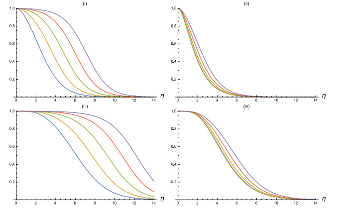
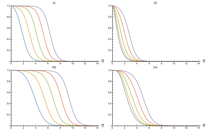
In Figures 5 and 6 some plots of $ {\cal R}(-\xi, \eta) $ are shown for $ \beta $ equal to 1 and 2, respectively, for $ \xi = 5 $ and for different choices of the parameters $ \alpha $ and $ \alpha^* $. As can be expected, the plots shows that $ {\cal R}(-\xi, \eta) $ is decreasing in $ \eta $ and $ \alpha^* $, increasing in $ \xi $ and $ \alpha $. Recall that the mean of $ U_i^+ $ and $ D_i^- $ is proportional to $ \alpha $ and $ \alpha^* $, respectively.
Among the generalizations of the classical telegraph process, the state-dependent versions are quite difficult to be treated. Differently from the analytical or transformation-based approaches adopted by various authors in the recent past, in this paper we exploited arguments of renewal theory to study the transition densities of a suitable family of state-dependent telegraph processes. We treated in detail the special case when certain random times of the motion have gamma distribution. This leads to an effective and treatable stochastic model. A specific feature is that consecutive velocity changes are separated by passages through the zero state. Such property yields that the considered process is suitable to describe fluctuating phenomena, such as the motion of particles that have alternating constant velocities and fluctuate around the origin. This can be a starting point toward the construction of more sophisticated models of interest in Neuroscience and in Biomathematics, which are based on stochastic processes whose sample-paths fluctuate around a time-varying signal or trend. Namely, a prototype stochastic model in this area can be expressed as
| $ Y(t) = s(t)+X(t), \qquad t\geq 0, $ |
where $ s(t) $ describes a suitable trend, such as a deterministic mean population growth, and $ X(t) $ is the stochastic component of the model that accounts for the fluctuations around the trend. The model of state-dependent fluctuations described in this paper can be adopted to deal with cases in which the system under investigation depends on the distance from the time-varying trend. Specific applications of this family of models will be the object of future investigation. Furthermore, possible future developments will be oriented to the construction of suitable tractable models in this area, also aiming to investigate the optimum signal determination with respect to the noise characteristics, by adopting suitable criteria as those exploited by Lansky et al. [41].
The constructive criticism of three anonymous referees is gratefully acknowledged.
The authors are members of the Research group GNCS of INdAM (Istituto Nazionale di Alta Matematica). This research is partially supported by MIUR - PRIN 2017, project "Stochastic Models for Complex Systems", no. 2017JFFHSH.
The authors declare no conflict of interest.
| [1] |
Roush SW, Murphy TV, Vaccine-Preventable Disease Table Working Group. (2007) Historical comparisons of morbidity and mortality for vaccine-preventable diseases in the United States. JAMA 298: 2155-2163. doi: 10.1001/jama.298.18.2155

|
| [2] | Lindberg C, Lanzi M, Lindberg K. (2015) Measles: Still a significant health threat. MCN Am J Matern Child Nurs 40(5): 298-305. |
| [3] |
Polgreen P M CY, Beekmann S E, Srinivasan A, Neill M A, Gay T, Cavanaugh J E. (2008) Elements of influenza vaccination programs that predict higher vaccination rates: Results of an emerging infections network survey. Clinical Infectious Diseases 46: 14-19. doi: 10.1086/523586
|
| [4] |
Zimmerman RK NM, Lin CJ, Raymund M, Fox DE, Harper JD, Tanis MD, Willis BC. (2009) Factorial design for improving influenza vaccination among employees of a large health system. Infect Control Hosp Epidemiol 30: 691-697. doi: 10.1086/598343
|
| [5] |
Ajenjo MC, Woeltje KF, Babcock HM, et al. (2010) Influenza vaccination among healthcare workers: ten-year experience of a large healthcare organization. Infect Control Hosp Epidemiol 31: 233-240. doi: 10.1086/650449
|
| [6] | Centers for Disease Control & Prevention (2011) Influenza vaccination coverage among health-care personnel--United States, 2010-11 influenza season. Morbidity and Mortality Weekly Reports 60: 1073-1077. |
| [7] |
Polgreen P M SEJ, Parry M F, Beekmann S E, Cavanaugh J E, Srinivasan A, et al. (2008) Relationship of influenza vaccination declination statements and influenza vaccination rates for healthcare workers in 22 U.S. hospitals. Infect Control Hosp Epidemiol 29: 675-677. doi: 10.1086/588590
|
| [8] |
Rebmann T, Wright KS, Anthony J, et al. (2012) Seasonal influenza vaccine compliance among hospital-based and nonhospital-based healthcare workers. Infect Control Hosp Epidemiol 33: 243-249. doi: 10.1086/664057
|
| [9] |
Rakita RM, Hagar BA, Crome P, et al. (2010) Mandatory influenza vaccination of healthcare workers: a 5-year study. Infect Control Hosp Epidemiol 31: 881-888. doi: 10.1086/656210
|
| [10] |
Ribner BS, Hall C, Steinberg JP, et al. (2008) Use of a mandatory declination form in a program for influenza vaccination of healthcare workers. Infect Control Hosp Epidemiol 29: 302-308. doi: 10.1086/529586
|
| [11] | Cole JP, and Swendiman, K. S. (2014) Mandatory Vaccinations: Precedent and current laws. Congressional Research Service. Avaiilable at: http://www.fas.org/sgp/crs/misc/RS21414.pdf. |
| [12] | California state. (2015) Public health: vaccinations. Health and Safety Code. Senate Bill No. 277. |
| [13] |
Babcock HM, Gemeinhart N, Jones M, et al. (2010) Mandatory influenza vaccination of health care workers: translating policy to practice. Clin Infect Dis 50: 459-464. doi: 10.1086/650752
|
| [14] | McCarty KL, Nelson GD, Hodge J, Jr., et al. (2009) Major components and themes of local public health laws in select U.S. jurisdictions. Public Health Rep 124: 458-462. |
| [15] | Kingdon JW. (2010) Agendas, Alternatives, and Public Policies. London: Pearson. |
| [16] | Coffman J (2007) The Evaluation Exchange: Evaluation Based on Theories of the Policy Process. Available at: http://www.hfrp.org/evaluation/the-evaluation-exchange/issue-archive/advocacy-and-policy-change/evaluation-based-on-theories-of-the-policy-process. |
| [17] | St. Louis County Department of Health. (2013) Mandatory hepatitis A vaccine ordinance for food handlers and subsequent decline in case rate in St. Louis County. Available at: http://www.naccho.org/topics/modelpractices/. |
| [18] | U.S. Census Bureau. (2000) 2000 Census. United States Government. |
| [19] | Centers for Disease Control & Prevention (1999) Prevention of hepatitis A through active or passive immunization: Recommendations of the Advisory Committee on Immunization Practices (ACIP). MMWR 48: 1-37. |
| [20] |
Craig AS, Watson B, Zink TK, et al. (2007) Hepatitis A outbreak activity in the United States: responding to a vaccine-preventable disease. Am J Med Sciences 334: 180-183. doi: 10.1097/MAJ.0b013e3181425411
|
| [21] |
Fiore AE. (2004) Hepatitis A transmitted by food. Clin Infect Dis 38: 705-715. doi: 10.1086/381671
|
| [22] | Potter J, Stott DJ, Roberts MA, et al. (1997) Influenza vaccination of health care workers in long-term-care hospitals reduces the mortality of elderly patients. J Infect Dis 175: 1-6. |
| [23] | Centers for Disease Control & Prevention (2015) Surveillance for Viral Hepatitis – United States, 2013. Available at: http://www.cdc.gov/hepatitis/statistics/2013surveillance/commentary.htm - hepatitisA. |
| [24] | Bohm S, R., Berger, K. W., Hackert, P. B., et al. (2015) Hepatitis A outbreak among adults with developmental disabilities in group homes — Michigan, 2013. MMWR 64: 148-152. |
| [25] |
Centers for Disease Control & Prevention. (2015) Pertussis epidemic-California, 2014. Ann Emerg Med 65: 568-570. doi: 10.1016/j.annemergmed.2015.02.009
|
| [26] | Missouri Department of Health. (2014) 2014-2015 Missouri school immunization requirements. Available at: http://www.nvic.org/Vaccine-Laws/state-vaccine-requirements/missouri.aspx. |
| 1. | Shuang Liang, Shenzhou Zheng, AN OPTIMAL GRADIENT ESTIMATE FOR ASYMPTOTICALLY REGULAR VARIATIONAL INTEGRALS WITH MULTI-PHASE, 2022, 52, 0035-7596, 10.1216/rmj.2022.52.2071 | |
| 2. | Dario Mazzoleni, Benedetta Pellacci, Calculus of variations and nonlinear analysis: advances and applications, 2023, 5, 2640-3501, 1, 10.3934/mine.2023059 | |
| 3. | Sun-Sig Byun, Ho-Sik Lee, Gradient estimates for non-uniformly elliptic problems with BMO nonlinearity, 2023, 520, 0022247X, 126894, 10.1016/j.jmaa.2022.126894 | |
| 4. | Maria Alessandra Ragusa, Atsushi Tachikawa, Regularity of minimizers for double phase functionals of borderline case with variable exponents, 2024, 13, 2191-950X, 10.1515/anona-2024-0017 | |
| 5. | Bogi Kim, Jehan Oh, Higher integrability for weak solutions to parabolic multi-phase equations, 2024, 409, 00220396, 223, 10.1016/j.jde.2024.07.012 | |
| 6. | Peter Hästö, Jihoon Ok, Regularity theory for non-autonomous problems with a priori assumptions, 2023, 62, 0944-2669, 10.1007/s00526-023-02587-3 | |
| 7. | Filomena De Filippis, Mirco Piccinini, Regularity for multi-phase problems at nearly linear growth, 2024, 410, 00220396, 832, 10.1016/j.jde.2024.08.023 | |
| 8. | Atsushi Tachikawa, Partial regularity of minimizers for double phase functionals with variable exponents, 2024, 31, 1021-9722, 10.1007/s00030-023-00919-y | |
| 9. | Jiangshan Feng, Shuang Liang, Regularity for Asymptotically Regular Elliptic Double Obstacle Problems of Multi-phase, 2023, 78, 1422-6383, 10.1007/s00025-023-02008-z | |
| 10. | Giuseppe Mingione, 2024, Chapter 2, 978-3-031-67600-0, 65, 10.1007/978-3-031-67601-7_2 | |
| 11. | Michela Eleuteri, Petteri Harjulehto, Peter Hästö, Bounded variation spaces with generalized Orlicz growth related to image denoising, 2025, 310, 0025-5874, 10.1007/s00209-025-03731-9 | |
| 12. | Bin Ge, Beilei Zhang, Campanato Type Estimates for the Multi-phase Problems with Irregular Obstacles, 2025, 22, 1660-5446, 10.1007/s00009-025-02849-8 | |
| 13. | Bogi Kim, Jehan Oh, Abhrojyoti Sen, Parabolic Lipschitz truncation for multi-phase problems: The degenerate case, 2025, 1864-8258, 10.1515/acv-2025-0003 |
Terri Rebmann, Kristin D. Wilson, Travis Loux, Ayesha Z. Iqbal, Eleanor B. Peters, Olivia Peavler. Outcomes, Approaches, and Challenges to Developing and Passing a Countywide Mandatory Vaccination Policy: St. Louis County’s Experience with Hepatitis A Vaccine for Food Service Personnel[J]. AIMS Public Health, 2016, 3(1): 116-130. doi: 10.3934/publichealth.2016.1.116

 DownLoad: