We consider nonlinear scalar conservation laws posed on a network. We define an entropy condition for scalar conservation laws on networks and establish $L^1$ stability, and thus uniqueness, for weak solutions satisfying the entropy condition. We apply standard finite volume methods and show stability and convergence to the unique entropy solution, thus establishing existence of a solution in the process. Both our existence and stability/uniqueness theory is centred around families of stationary states for the equation. In one important case – for monotone fluxes with an upwind difference scheme – we show that the set of (discrete) stationary solutions is indeed sufficiently large to suit our general theory. We demonstrate the method's properties through several numerical experiments.
Citation: Markus Musch, Ulrik Skre Fjordholm, Nils Henrik Risebro. Well-posedness theory for nonlinear scalar conservation laws on networks[J]. Networks and Heterogeneous Media, 2022, 17(1): 101-128. doi: 10.3934/nhm.2021025
We consider nonlinear scalar conservation laws posed on a network. We define an entropy condition for scalar conservation laws on networks and establish $L^1$ stability, and thus uniqueness, for weak solutions satisfying the entropy condition. We apply standard finite volume methods and show stability and convergence to the unique entropy solution, thus establishing existence of a solution in the process. Both our existence and stability/uniqueness theory is centred around families of stationary states for the equation. In one important case – for monotone fluxes with an upwind difference scheme – we show that the set of (discrete) stationary solutions is indeed sufficiently large to suit our general theory. We demonstrate the method's properties through several numerical experiments.

| [1] |
Well-posedness for vanishing viscosity solutions of scalar conservation laws on a network. Discrete Contin. Dyn. Syst. (2017) 37: 5913-5942. 
|
| [2] |
B. P. Andreianov, G. M. Coclite and C. Donadello, Well-posedness for a monotone solver for traffic junctions, preprint, arXiv: 1605.01554. |
| [3] |
A Theory of $L^1$-dissipative solvers for scalar conservation laws with discontinuous flux. Arch. Ration. Mech. Anal. (2011) 201: 27-86.
|
| [4] |
Uniqueness for scalar conservation laws with discontinuous flux via adapted entropies. Proc. Roy. Soc. Edinburgh Sect. A (2005) 135: 253-265.
|
| [5] |
Convergence rates of monotone schemes for conservation laws with discontinuous flux. SIAM J. Numer. Anal. (2020) 58: 607-629.
|
| [6] |
Flows on networks: Recent results and perspectivees. EMS Surv. Math. Sci. (2014) 1: 47-111.
|
| [7] |
An Engquist–Osher-type scheme for conservation laws with discontinuous flux adapted to flux connections. SIAM J. Numer. Anal. (2009) 47: 1684-1712.
|
| [8] |
G. M. Coclite and L. di Ruvo, Vanishing viscosity for traffic on networks with degenerate diffusivity, Mediterr. J. Math., 16 (2019), Paper No. 110, 21 pp. |
| [9] |
Vanishing viscosity on a star-shaped graph under general transmission conditions at the node. Netw. Heterog. Media (2020) 15: 197-213.
|
| [10] |
Vanishing viscosity for traffic on networks. SIAM J. Math. Anal. (2010) 42: 1761-1783.
|
| [11] |
Some relations between nonexpansive and order preserving mappings. Proc. Amer. Math. Soc. (1980) 78: 385-390.
|
| [12] |
One-sided difference approximations for nonlinear conservation laws. Math. Comp. (1981) 36: 321-351.
|
| [13] |
U. S. Fjordholm, M. Musch and N. H. Risebro, Well-posedness of traffic flow models on networks, Submitted to SIAM Journal on Numerical Analysis, 2021. |
| [14] |
A review of conservation laws on networks. Netw. Heterog. Media (2010) 5: 565-581.
|
| [15] | Entropy type conditions for Riemann solvers at nodes. Adv. Differential Equations (2011) 16: 113-144. |
| [16] | A difference method for numerical calculation of discontinuous solutions of the equations of hydrodynamics.. Mat. Sb. (1959) 47: 271-306. |
| [17] |
H. Holden and N. H. Risebro, Front Tracking for Hyperbolic Conservation Laws, 2$^{nd}$ edition, Springer-Verlag, Berlin, Heidelberg, 2015. |
| [18] |
A mathematical model of traffic flow on a network of unidirectional roads. SIAM J. Math. Anal. (1995) 26: 999-1017.
|
| [19] |
K. H. Karlsen, N. H. Risebro and J. D. Towers, $L^1$-stability for entropy solutions of nonlinear degenerate parabolic convection-diffusion equations with discontinuous coefficients, Skr. K. Nor. Vidensk. Selsk., (2003), 1–49. |
| [20] |
Upwind difference approximations for degenerate parabolic convection-diffusion equations with a discontinuous coefficient. IMA J. Numer. Anal. (2002) 22: 623-664.
|
| [21] | First order quasilinear equaitons in several independent variables. Mat. Sb. (N.S.) (1970) 81: 228-255. |
| [22] |
Accuracy of some approximate methods for computing the weak solutions of a first-order quasi-linear equation. USSR Computational Mathematics and Mathematical Physics (1976) 16: 105-119.
|
| [23] |
On kinematic waves Ⅱ. A theory of traffic flow on long crowded roads. Proc. Roy. Soc. London Ser. A (1955) 229: 317-345.
|
| [24] |
Riemann solvers, the entropy condition, and difference approximations. SIAM J. Numer. Anal. (1984) 21: 217-235.
|
| [25] |
Existence of strong traces for quasi-solutions of multidimensional conservation laws. J. Hyperbolic Differ. Equ. (2007) 4: 729-770.
|
| [26] |
Waves on the highway. Operations Res. (1956) 4: 42-51.
|
| [27] |
A convergent finite difference scheme for the Ostrovsky–Hunter equation with Dirichlet boundary conditions. BIT Numerical Mathematics (2019) 59: 775-796.
|
| [28] |
Global solution of the Cauchy problem for a class of $2\times 2$ nonstrictly hyperbolic conservation laws. Adv. in Appl. Math. (1982) 3: 335-375.
|
| [29] |
J. D. Towers, An explicit finite volume algorithm for vanishing viscosity solutions on a network, Netw. Heterog. Media, 2021. |
| [30] |
Convergence of a difference scheme for conservation laws with a discontinuous flux. SIAM J. Numer. Anal. (2000) 38: 681-698.
|
Figures(4) / Tables(1)
Markus Musch, Ulrik Skre Fjordholm, Nils Henrik Risebro. Well-posedness theory for nonlinear scalar conservation laws on networks[J]. Networks and Heterogeneous Media, 2022, 17(1): 101-128. doi: 10.3934/nhm.2021025

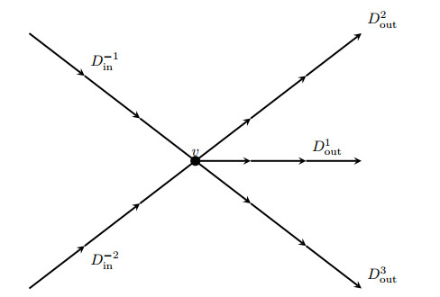
A star shaped network with two ingoing and three outgoing edges
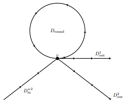
A network with a periodic edge
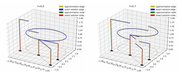
Initial state and state at
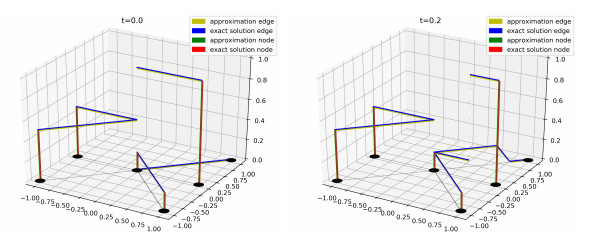
Initial state at


 DownLoad: