Analysis of a system of nonlocal conservation laws for multi-commodity flow on networks

1.   Introduction

Recently, bioimpedance spectroscopy (BIS) is found to have tremendous applications in medical sciences, especially in physiological diagnosis. The major application area of BIS is detection of various diseases including cancer. The first step in experimental study of BIS is the measurement of bioimpedance (of the biological body under question) as a function of frequency. The measured bioimpedance elucidates the electrical characteristics of biological tissue. In the next step, Cole parameters are extracted by fitting the measured bioimpedance data, and finally, the biological tissue or body under investigation is described in terms of Cole parameters. The Cole model [1] is the most accepted and widely-used impedance model to describe biological tissue or body. As the values of the Cole parameters are highly dependent on the cell membranes and quantity of the intracellular and extracellular fluid, the parameters of the Cole model provide essential information in characterizing the properties of biological tissue, and it is extensively used for practical purposes which include determining human body composition [2],[3], discriminating tissues of fruit or vegetable [4], the effect of moisturizing cream on human skin [5], characterization of prostate cancer [6], the effect of storage conditions [7], physiological changes including determining the vegetable quality [8], etc.

The most efficient optimization method for extracting the Cole parameters is scientifically not proven with rigorous and robust analyses of the properties of biological tissue. The gradient-based NLS algorithm is the most conventional optimization technique to fit the BIS data and extract the Cole parameters [9],[10]. The NLS algorithm is well known for its computational simplicity, faster runtime, availability and its wide applicability. Unfortunately, the optimization performance of this algorithm is unsatisfactory against the existence of noise and outliers in the measured BIS data, which in turn affects the precision of the estimated Cole parameters. Because the outcome of the fitting of this approach is strongly dependent on the solution vector's starting values, it is prone to converge in local minima frequently. Therefore, the NLS algorithm is not a reliable choice for extracting the Cole parameters accurately; hence, more efficient algorithms are required. Finding efficient algorithms to estimate Cole parameters from measured BIS data is the objective of this present work.

On the other hand, nature-inspired optimization algorithms are implemented for various real-world problems due to their remarkable optimizing capabilities. These algorithms are designed by simulating various natural intelligent behaviour demonstrated by several creatures. In general, these algorithms start with a set of random solutions, and then this set is improved by using mathematical equations inspired by nature. Due to the usage of multiple solutions, these algorithms can search more areas in the search space. So, if any search agent is trapped in a local solution, other search agents can search for the global solution. Another fundamental feature of these algorithms is the use of stochastic components. These components allow the algorithms to fluctuate the search agents in a randomized manner, increasing the chance of finding the optimal solution. Changing the magnitude of random components during the optimization process leads the algorithms to a systematic stochastic search. Due to these advantages, many such algorithms are implemented in a large number of popular areas such as optimizing neural networks [11], spam and intrusion detection systems [12],[13], breast cancer detection [14], Internet of Things (IoT) [15], geographic atrophy segmentation for SD-OCT images [16], power dispatch problems [17], image segmentation [18], antenna array design [19], PID controller design [20], aerospace technology [21], terrorism prediction [22], finding neural unit modules for brain network [23] protein structure prediction [24] etc. These capabilities of nature-inspired algorithms naturally demand their applicability in the estimation of Cole parameters from measured BIS data.

In this paper, a novel and robust process is presented to estimate Cole parameters accurately. Six different nature-inspired optimization algorithms are used to extract the Cole parameters and compare the algorithms' efficiency with the conventional NLS algorithm. Six nature-inspired algorithms used in this work are Cuckoo Search (CS) algorithm [25],[26], Grey Wolf Optimization (GWO) [27], Moth Flame Optimization (MFO) [28], Particle Swarm Optimization (PSO) [29],[30], Sine Cosine Algorithm (SCA) [31] and Whale Optimization Algorithm (WOA) [32]. The effectiveness of all algorithms is evaluated over the sets of both simulated BIS data where the noise has been injected intentionally into the dataset, as well as the measured BIS data of different root vegetables for analyzing the change in physiological properties due to the aging effect. The root vegetables selected for this study are Ginger (Zingiber officinale), Potato (Solanum tuberosum) and Sweet Potato (Ipomoea batatas). This research work aims to investigate the robustness of each proposed algorithm against unwanted noise and determine the most efficient algorithm to gain statistical relevance using a minimum sample size. In the case of simulated BIS data, the CS algorithm showed the best-fit result in terms of noise immunity and achieved the highest precision in terms of the extracted Cole parameters. For measured BIS data of the root vegetables, ANOVA is performed on the relaxation time estimated from the extracted Cole parameters between the first and final day data measurement for each algorithm. The experimental results illustrate that the CS algorithm achieved the highest efficiency among all the algorithms, using a minimum sample size to gain statistical relevance. In this work, all algorithms are implemented using Python programming language and ANOVA is performed using the standard libraries available in Microsoft Excel.

2.   Cole bioimpedance model and extraction of Cole parameters

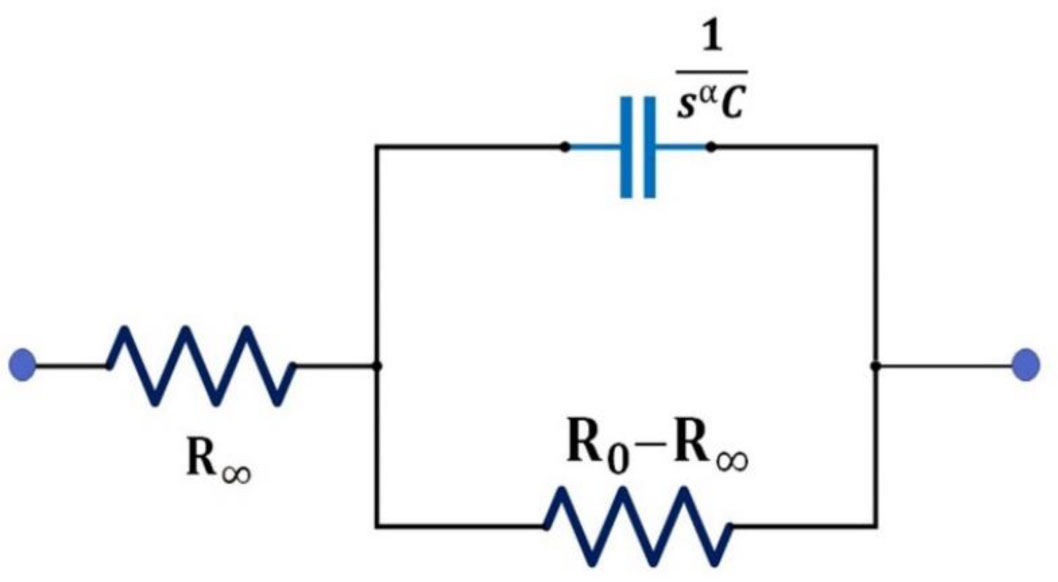
The Cole bioimpedance model [1,4,5] is the most well-known model used for the characterization of biological tissue. Figure 1 represents the equivalent circuit of the Cole bioimpedance model. From the equivalent circuit, it can be seen that the tissue behaves like an RC series-parallel circuit where a resistance R_∞ is connected in series with a parallel combination of a fractional capacitor (C) and a resistance (R₀ − R_∞) (see Figure 1).

Figure 1.  Cole equivalent circuit for biological tissue.

DownLoad: Full-Size Img PowerPoint

The mathematical expression for Cole impedance is:

where, j=−1, R₀ indicates the impedance at very low frequency, R_∞ indicates the impedance at very high frequency, ω indicates the angular frequency, α indicates the dimensionless exponent (0 < α < 1 for biological tissue) and τ indicates the relaxation time of the tissue and Eq. (2) represents the mathematical expression of τ.

The mathematical expression of the real and imaginary components of Z is represented using Eq. (3) and (4) [33].

The modulus of the impedance Z is represented by:

A typical Cole plot (negative of the imaginary part of the impedance along vertical axis and real part of the impedance along the horizontal axis as a function of frequency, also known as Nyquist plot in the discipline of electronics) looks like a semi-circle (but practically not exactly semi-circle) and is schematically shown in Figure 2.

Figure 2.  Typical Cole plot (or Nyquist plot).

DownLoad: Full-Size Img PowerPoint

The mathematical equation of the impedance locus in Figure 2 is represented using Eq. (6) [33].

Eq. (6) is an equation of a circle whose centre lies below the horizontal axis and mathematical expressions of centre of the circle and radius of circle are represented using Eq. (7) and (8) [33].

The mathematics of separating the real and imaginary parts of impedances can also be found in standard references [4],[5]. Experimentally |Z| and the phase angle is measured in the frequency range of 1 Hz to 50 kHz. Then the Cole parameters [R₀, R_∞, α, c] are obtained by fitting the experimental data with the theoretical Cole impedance expressed by Eq. (5). In this fitting process, various algorithms are investigated. In order to fit experimental BIS data, the objective function is defined as the sum of the squared error (SSE) between the complex observed impedance and the predicted impedance from Eq. (5). The mathematical representation of the objective function is represented using Eq. (9).

where, Z(x, f_j) is the measured impedance at frequency f_j, Z^j is the estimated impedance at frequency f_j, x represents the set of Cole parameters [R₀, R_∞, α, c] and n is the number of frequency points (or simply number of data points). To reduce the complexity of the above equation, the real and imaginary components are separated using Eq. (10).

where, ℜ{·} and ℑ{·} indicates the real and imaginary components of impedance respectively.

Finally, the Cole parameters [R₀, R_∞, α, c] are evaluated by the minimization or optimization of the objective function (SSE). During this process, the Cole parameters act as solution vector (X). The lower and upper boundaries of each parameter [X_L, X_H] represent the search space of the optimization process. At the starting of every algorithm, the initial values of the parameters are calculated using Eq. (11).

where, X_i,0 indicates the initial values for the solution vector (X) and rand is a randomly generated value between the interval [0,1]. After initialization, every optimization algorithm uses their unique mathematical techniques to extract the global values of the Cole parameters by minimizing the objective function.

3.   Experimental protocol and measurement

In order to get electrical access into biological samples (Potato, Sweet Potato, Ginger), an electrode-pair is designed and fabricated. Figure 3 represents a schematic diagram of the fabricated electrode-pair. Using a disposable syringe, the mounting structure of the electrode-pair is made. Stainless steel is chosen for the electrode material as it is reluctant to react with any other material and provides adequate strength at a low wire diameter. Electrode made of a material which reacts with biological tissue will definitely yield erroneous results and such electrode should be avoided. The distance between the electrodes is 3 mm, and the diameter of the electrodes is 0.28 mm. Throughout this work, the penetration depth is kept at 1.5 cm for maintaining identical conditions during measurement. A similar experimental procedure can also be found in standard reference [4] on bioimpedance measurement. As the Cole parameters (except α) are highly dependent on the distance between the two electrodes, this separation is kept constant throughout the experiment. It is to be noted here that for a given biological body, the relaxation-time (τ) is independent of the distance between the electrodes and it is a characteristic parameter of the biological body.

Figure 3.  Schematic diagram of the fabricated electrode-pair.

DownLoad: Full-Size Img PowerPoint

We have used a 1 MHz precision LCR meter (Model: 8101G, Make: GW Instek) to measure the root vegetables' BIS data. The LCR meter is calibrated before taking any BIS data measurement to remove any parasitic effect. Before penetrating the electrode pairs inside the root vegetables, the electrodes are cleaned by the medicated spirit and dried appropriately every time. The LCR meter measures the magnitude of impedance and corresponding phase angle using a sinusoid of 1 V (peak-to-peak) over a frequency range from 1 Hz to 50 kHz with 200 steps. The measured data is recorded by a PC connected with the LCR meter through an RS-232C serial port.

In order to get experimental BIS data, three commonly available root vegetables, i.e., potato, sweet potato and ginger, are considered as biological samples in this study. To analyze the efficiency of each proposed algorithm in various BIS data distribution ranges, these specific root vegetables are selected for this work as their Cole parameters are located at different BIS data distribution ranges from each other. The entire BIS data measurement system of the root vegetables is shown in Figure 4. The change in physical properties due to the aging effect of specific root vegetables using Cole parameters from measured BIS data is analysed. The BIS measurement is conducted for up to twelve days, maintaining a gap of one or two days for each sample. For each measurement day, five different measurements of bioimpedance are recorded for every biological sample. Thus, a total of 30 datasets (6 days × 5 positions) for each biological sample is measured at a controlled temperature of 25 °C and 70% humidity. The measurement period and its timeline are illustrated in Figure 5.

Figure 4.  Experimental setup.

DownLoad: Full-Size Img PowerPoint

Figure 5.  Pictorial depiction of measurement timeline.

DownLoad: Full-Size Img PowerPoint

Each bioimpedance measurement generates a single set of BIS data which contains two hundred data points. As the numerical values of biological tissue-related parameters vary with a large standard deviation due to the diversity of the cell size, five such bioimpedance measurement at five different positions of each biological sample has been recorded in our study. For vividly analysing the change in physical properties, only the first and final day data measurement of each root vegetable is considered for the Cole parameter extraction. Consequently, there are ten datasets in total for each biological sample to analyse the aging effect of root vegetables. For the convenience of the fitting process, from two hundred data points, only fifty data points are selected manually (using loop in python), which are distributed at approximately equal distances from each other in imaginary impedance and real impedance space. As the relaxation time (τ) contains all the Cole Parameters (see Eq. (2)), it is the most important tissue characterizing parameter [4,5]. Hence, the relaxation time is calculated using Eq. (2) for each case and is used to perform an ANOVA to gain statistical relevance for each root vegetable.

4.   Optimization algorithms

4.1.   Non-linear least square optimization

The least-square optimization is the most widely used method for fitting any linear or non-linear curve by minimizing the sum of squared residuals of a set of data points from the plotted curve. There are two types of least-square optimization; one is ordinary or linear least-square optimization, where the residuals are linear, and the non-linear least-square optimization, where the residuals are non-linear. The main objective of this method is to find the optimum value of parameters of a model function to fit the curve in the best possible way.

Suppose, for an optimization problem, the data points are (m₁, n₁), (m₂, n₂), (m₃, n₃), ..., (m_j, n_j) in which m is the independent variable and n is the dependent variable whose values are found by observation (through experiment). Here the model function is defined as f(m, β), where β is the parameter of the model function, the value of which is to be optimized. The sum of squared residuals (S) of the data points are defined using Eq. (12).

The least-square optimization method finds the optimal value of β by minimizing S. The minimum of S is found by calculating its gradient with respect to β and setting the gradient to zero.

The NLS algorithm is directly implemented by using the built-in least squares available function in a python module named scipy [34]. In the least squares function, the value of maximum iteration is adjusted by the requirements of the objective function through an internal method by default. Hence, we cannot change the number of maximum iterations.

4.2.   Cuckoo search optimization

The CS algorithm was introduced by Xin-She Yang and Suash Deb [25], which is inspired by the brood parasitism of cuckoos in combination with the Lévy flight behaviour of specific birds and fruit flies. Cuckoos are a family of birds who adopted a unique egg-laying strategy to increase the survival rate of their species. Some cuckoo species, such as the Ani and Guira, lay their eggs in the nests of birds of different host species. If the host birds realise that the eggs are not their own, they can participate in a direct fight with the intruding cuckoos and throw those alien eggs away, or they can abandon their nest and construct a new one. Several cuckoo species have evolved due to this, like Tapera, which can imitate the host birds' colour and pattern of eggs. Even some cuckoo chicks can mimic the call of host chicks, which increases the survival rate of the cuckoo species.

In the CS optimization algorithm, each egg in a host bird's nest represents a solution in d-dimensional search space; each cuckoo can only lay one egg at a time. The goal is to replace a poor solution in the nests with a new and better one. In this algorithm, there is no distinction between a cuckoo, an egg, or a nest because each cuckoo corresponds to one egg representing one nest, corresponding to a single solution vector in d-dimensional search space. At first, in this optimization process, each cuckoo lays one egg and then dumps it in a random nest. Then, the best nests representing the best solutions will be carried over to the subsequent iterations. The probability of discovering a cuckoo's egg by the host bird is p_a ∈ [0,1]. Hence, a fraction p_a of the n host nests is substituted by new nests, representing new randomly generated solutions.

In this algorithm, both the local and global explorative random walk are manipulated by a switching parameter p_a. The mathematical equation of local random walk is represented using Eq. (13) [26].

where, H(u) indicates a Heaviside function, ε indicates a random number generated from a uniform distribution, s is the step size, β is a small scaling factor, xjt and xkt are two different randomly selected solutions by random permutation. The mathematical equation of the global random walk, which is carried out by using Lévy flights is represented using Eq. (14) [26].

Here, α indicates the step size scaling factor, ⊗ denotes an entry-wise operation and L(s, λ) is the power-law distribution. The notation ‘∼’ indicates that the random numbers L(s, λ) must be drawn from the Lévy distribution on the right-hand side with an exponent λ. The gamma function (Γ) is defined using Eq. (16).

4.3.   Grey wolf optimization

The population-based GWO algorithm was introduced by Mirjalili [27], which is inspired by the behaviour of the grey wolves in nature. In order to search for the optimal solution, the GWO algorithm imitates the social hierarchy and the intelligent hunting strategy of grey wolves. According to their social hierarchy, there are four types of grey wolves: alpha, beta, delta and omega. Every type of grey wolf plays a different role in hunting, involving three significant actions: seeking prey, encircling prey and attacking the prey.

Considering the domination level, there are four different types of members: alpha, beta, delta and omega in a pack of wolves. Alpha is the most dominant wolf in the group, responsible for making most of the decisions, and other wolves obey the decisions made by alpha. Beta wolves come next to the alpha in the leadership hierarchy of grey wolves, and they help the alpha make decisions. The delta wolves come next in this domination level, and they act as scouts, sentinels, and caretakers in the pack. The weakest class of domination in a pack of wolves is the omega which follows every decision made by other wolves. To implement this system mathematically in the GWO algorithm, the first three best solutions are considered as α, β, δ and the rest of the solutions are considered as ω. After this consideration, the position of grey wolves (search agents) is updated using the following mathematical models.

Encircling Prey: At first, grey wolves chase the prey in a team, then encircle the prey by changing their position with respect to the prey's movement direction. The mathematical model of this encircling behaviour is represented using Eq. (17) and (18) [27].

where, t indicates the current iteration number, X→ indicates the position of a grey wolf, Xp→ indicates the position of the pray, D→ indicates the new position of the grey wolf, A→ and C→ are the coefficient vectors which forces the wolves to diverge from the prey to emphasize the global search. A→ and C→ can be calculated using Eq. (19) and (20) [27].

where, a→ is a parameter which decreases linearly from 2 to 0 with increasing iteration and r₁, r₂ are randomly generated value from the interval [0,1]. The mathematical equation to update parameter a is represented using Eq. (21) [27].

where, T indicates the total number of iterations.

Hunting the Prey: After locating and encircling the prey, the alpha usually guides the hunting mechanism. In GWO, the alpha, beta and delta are considered the first three optimum solutions obtained so far, which is an essential consideration because other search agents (omega wolves) improve their positions following to the position of the best search agents. The position of each wolf is updated over the iteration using Eq. (22), (23), and (24) [27].

where, Xα→, Xβ→ and Xδ→ are the current position of alpha, beta and delta wolf, respectively and Dα→, Dβ→ and Dδ→ are the new position of alpha, beta and delta wolf, respectively.

4.4.   Moth flame optimization

The population-based MFO algorithm was introduced by Mirjalili [28], which is inspired by the navigating mechanism of moths at night using a light source known as transverse orientation. When moths travel at night, they maintain a fixed angle with respect to the moon during flying. As the distance from the earth to the moon is very large (384,400 km), this effective mechanism helps the moths to travel long distances in a straight line. However, in the presence of artificial light sources such as electric lamps or candles, the transverse orientation creates a converging spiral path around the light source as the distance is much smaller compared to the moon.

In the MFO algorithm, a population of n-moths work as search agents. Each moth contains a d-dimensional vector corresponding to the problem's solution, and the flames are denoted as flags assigned by moths in the d-dimensional search space. Each moth moves around in the d-dimensional space, and the possible solutions are the positions of the moths. In each cycle, a nominal moth hunts around a flame for a better solution, and when one is discovered, it changes the flame's location. The MFO algorithm contains three parts which are defined using Eq. (25) [28].

where, I is the initialization function for generating a set of random population of moths between the upper and lower boundaries of the decision variables and their corresponding fitness values defined using Eq. (26) and (27) [28].

where, i indicates the number of moths, j indicates the number of flames and ub, lb are the upper and lower boundaries of the decision variables, respectively. P is the primary function of this algorithm, by which the moths travel around the d-dimensional search space. Until the T termination function is achieved, the P function receives the matrix of M and returns its updated values on each iteration. The mathematical equation of the logarithmic spiral function is selected to imitate the transverse orientation of moths is represented using Eq. (28) and (29) [28].

where, S is the spiral function, M_i indicates the i^th moth and F_j indicates the j^th flame. D_i is the distance between the i^th moth and j^th flame, b is a constant which determines the shape of the logarithmic spiral and t indicates a random number in [r,1], where r is convergence constant which linearly decreased from −1 to −2 with increasing iteration for accelerating the convergence speed. Lower value of t indicates the closer distance from moth to the flame.

The number of flames is lowered adaptively during the iterations to address the problem of diminishing the exploitation of the best promising option. The mathematical equation of this adaptive flame reduction during every iteration is represented using Eq. (30) [28].

where, N indicates the initial number (or maximum number) of flames, l indicates the current number of iterations and T indicates the total number of iterations.

4.5.   Particle swarm optimization

The meta-heuristic Particle Swarm Optimization (PSO) algorithm was introduced by Kennedy and Eberhart [29], which is inspired by the flocking behaviour of birds in nature. In this algorithm, a population of n particles acts as search agents in the d-dimensional search space, where each particle contains a solution vector of a given optimization problem. The search agents travel in the d-dimensional search space by updating their position at every iteration to find the global solution. The algorithm mainly consists of two vectors: the position vector and the velocity vector. The position vector defines the current position, and the velocity vector represents the direction and magnitude of step size for each dimension and each search agent independently. The position of the search agents is updated in every iteration using Eq. (31) [30].

where, X_i(t) indicates the position of the i^th particle at t^th iteration and V_i(t) indicates the velocity of the i^th particle at t^th iteration. The mathematical equation of the velocity vector of the particles is represented using Eq. (32) [30].

where, w indicates the inertial weight, c₁ indicates the individual coefficient, c₂ indicates the social coefficient and r₁, r₂ are random numbers between the interval [0,1], P_i(t) indicates the best solution obtained by the i^th particle until the t^th iteration and G(t) indicates the best solution obtained by all particles until the t^th iteration.

According to Eq. (32), there are three components in the velocity vector responsible for the movement of particles in the d-dimensional search space. The first component wVi(t)→ is responsible for the contribution towards the previous velocity. This contribution depends on the inertial weight (w). A larger value of this parameter means a higher affinity to maintain the previous velocity. The second component c1r1(Pi(t)→−Xi(t)→) maintains the tendency towards the best solution that a particle has obtained so far. The individual coefficient c₁ and random number r₁ manipulate the tendency towards the best solution of a particle until the t^th iteration. Finally, the third component c2r2(G(t)→−Xi(t)→) maintains the tendency around the best solution found by all particles until the t^th iteration. The social coefficient c₂ and random number r₂ manipulate the impact of this component.

4.6.   Sine cosine algorithm

The population-based SCA was introduced by Mirjalili [31], which is developed by two main mathematical equations. The equations are represented using Eq. (33) and Eq. (34) [31].

where, t indicates the current iteration number, Xit+1 indicates the position of the i^th search agent in the (t + 1)^th iteration, Xit indicates the position of the i^th search agent in the t^th iteration, r₁ represents a random number which defines the magnitude of the range of sin and cosine function, r₂ represents a random number which defines the domain of the sin and cosine function and r₃ represents a random number which indicates the magnitude of the destination contribution for reaching a new position to the global minima. As the usage of sine and cosine functions play a vital role in these equations, this algorithm has been named Sine Cosine Algorithm. The combination of using these two equations is represented using Eq. (35) [31].

where, r₄ is a random number between the interval [0,1]. All these random variables play a crucial role in SCA. The parameter r₁ is responsible for changing the magnitude of the range of sin and cosine function, which is the primary mechanism to move the search agents towards or outwards the destination. With increasing iteration, the parameter r₁ is linearly decreased in SCA represented using Eq. (36) [31].

where, a is a constant and T indicates the total number of iterations. Similarly, the second parameter r₂ is responsible for changing the step size of a search agent towards or outwards the destination. The third parameter r₃ indicates the contribution level of the destination, and this contribution reduces with increasing the iteration number. Finally, the fourth parameter r₄ allows SCA to choose between the sin and cosine function with an equal probability.

4.7.   Whale optimization algorithm

The meta-heuristic Whale Optimization Algorithm (WOA) was introduced by Mirjalili [32], which was inspired by the bubble-net foraging behaviour of humpback whales. Due to their considerable bodyweight, humpback whales need to consume a massive number of fish or krill regularly. For this reason, they adopted an evolutionary process to trap prey in a specific place as they are not fast enough to chase. In this process, when the humpback whales detect a school of krill or small fishes, they swim in a spiral-shaped path around the prey while making bubbles. When the school of krill or small fishes move towards the surface, humpback whales attack them.

In WOA, a population of n whales act as search agents in the d-dimensional search space, with each whale containing a solution. The search agents travel in the d-dimensional search space by updating their position in every iteration to find the global minima. The mathematical representation of this position update method is represented using Eq. (37) and (38) [32].

where, X→(t) represents the position of the search agent at t^th iteration, X*→(t) indicates the possible position of the prey at t^th iteration, D→ indicates the distance between the whale and the prey, A→ and C→ are the coefficient vectors which force the whales to diverge from the prey to emphasize the global search. The mathematical equations of these coefficient vectors are represented using Eq. (39) and (40) [32].

where, a→ is a parameter which decreases linearly from 2 to 0 with increasing iteration and r1→, r2→ are random vectors in the interval [0,1]. Eq. (37) allows the search agents to travel any areas around a given prey (X*(t)) and the random vectors help the search agents to move in a hyper-rectangle space around the prey. The mathematical representation of the spiral movement of whales in the WOA, is represented using Eq. (41) [32].

where, b represents a constant value used to define the shape of the logarithmic spiral, l represents a random number in the interval [−1,1] and D′→ indicates the best solution obtained so far. As the humpback whales simultaneously swim around a spiral-shaped path and a shrinking circle around the prey, the probability of choosing between the spiral path or shrinking encircling mechanism is 50%. The mathematical representation of this simultaneous behaviour is represented using Eq. (42) [32].

where, p is a random number in the interval [0,1].

5.   Extraction of Cole parameters from simulative experiments

5.1.   Preparation of datasets for simulation

In order to verify the accuracy of the proposed optimization algorithms, a large number of data is generated through simulation and Cole parameters are extracted using those algorithms with predefined sets of parameters. For the detail accuracy comparison, simulated datasets are generated using three different sets of Cole parameters. Further, two different levels of random noise (0 to ± 5 % and 0 to ± 10 %) are introduced in each dataset. Thus, a total of six different sets of simulated datasets are generated and considered for investigation. The entire dataset matrix is shown in Table 1. In our tables, 1EX represents 10^X.

Table 1.  Specification of the Cole parameters for simulated datasets.

Set No.	R0 (Ω)	R∞ (Ω)	α	C (Fsα-1)	Random Noise
1	8350	450	0.65	1.5E-07	5%
2	8350	450	0.65	1.5E-07	10%
3	12500	600	0.7	4.0E-08	5%
4	12500	600	0.7	4.0E-08	10%
5	18550	750	0.75	2.0E-08	5%
6	18550	750	0.75	2.0E-08	10%

---

 | Show Table

DownLoad: CSV

Each simulated dataset consists of 50 distributed frequency points (f₁, f₂ ... f₅₀) ranging from 1 Hz to 50 kHz. The chosen dataset values of Cole parameters are based on some typical range of Cole parameters of root vegetables. The random noises in the datasets are imposed using the mathematical equations are represented using Eq. (43) and (44) [10].

where, (x_ri, y_ri) is the reference simulated data evaluated from Eq. (3) and (4), rand is a random number with continuous uniform distributions between the interval [−1,1], r₀ is the radius of the Cole plot evaluated from Eq. (8) and the value of the coefficient β is 0.05 when the random noise level is 5%, or 0.1 when the random noise level is 10%. Here θ_i indicates the angle between the horizontal axis and the radial direction. The mathematical representation of θ_i is represented using Eq. (45) [10].

where, (x₀, y₀) represents the centre of the circle of Cole Plot.

5.2.   Simulation procedure

To implement this experiment, Python programming language is used to write every algorithm, and the Google Colabotary cloud platform is used to run every algorithm. Except for NLS, functions for optimizing the objective function of all the nature-inspired algorithms are written manually using their mathematical models and implemented in the python programming language. Throughout the experiment, the population size is set to 100 and the maximum iteration is set to 1000 for each algorithm. The same upper and lower boundaries of the Cole parameters [R₀, R_∞, α, c] are maintained for all the algorithms, which are:

In the case of the NLS algorithm, the parameters extracted by the algorithm consisted of several non-realistic values, which imply the negative capacitance of the Cole model. To avoid these non-realistic values in NLS, all the invalid solutions are rejected and only the realistic solutions are considered for accuracy comparison.

As the random noise generation is different (randomly) at every algorithm runtime, simulated BIS data points distribution differs. This problem of the randomness of fitting performance is avoided by running ten times for each dataset for every algorithm. The mean and standard deviation of the extracted Cole parameters are considered to evaluate the fitting performance of a given optimization algorithm. Also, for better evaluation, the mean and standard deviation of the percentage error of the Cole parameters [R₀, R_∞, α, c] are estimated and compared for every dataset.

6.   Results and discussion

The first portion of this section contains results the from simulation, while the second portion contains results from our experimentation. Simulation results are obtained for seven optimizing algorithms. Every algorithm is executed for six different data sets and ten independent runs for a given data set. As a representative, the best fit result of ten independent runs for the seven optimization algorithms on each data set is shown in Figure 6.

Figure 6.  Simulated real vs imaginary impedance fitting curve along with the BIS data points. (a) Set–1; (b) Set–2; (c) Set–3; (d) Set–4; (e) Set–5; (f) Set–6.

DownLoad: Full-Size Img PowerPoint

The results from the simulated data sets are tabulated in Table 2 to Table 7. The mean, standard deviation (SD), error percentage of mean and percentage error of the standard deviation of the Cole parameters [R₀, R_∞, α, c] of ten independent executions for every algorithm on the six different simulated datasets are presented in these tables. In addition to this, we have computed the regression coefficients of the curve fitting process and execution time taken by each algorithm for each run. The average runtime (average of ten run) and average regression coefficient (average of ten) for the six simulated datasets are shown in Table 8 and Table 9, respectively.

Table 2.  Fitting result for dataset–1.

Algorithm	Cole Parameter	Mean	SD	Mean (% Error)	SD (% Error)
CS	R0	8355.107	43.60109	0.465499	0.18987
	R∞	442.4472	82.89779	13.86056	11.3591
	c	1.53E-07	1.07E-08	5.752247	4.345003
	α	0.648145	0.008704	1.047105	0.815723
GWO	R0	8516.781	106.3356	2.05287	1.171322
	R∞	174.1789	189.1883	66.50499	32.05469
	c	1.98E-07	2.98E-08	32.61239	18.32311
	α	0.616692	0.020714	5.363011	2.715322
MFO	R0	8360.918	38.99457	0.399048	0.245265
	R∞	434.6529	63.47616	12.20855	6.803532
	c	1.52E-07	8.5E-09	4.775471	2.935314
	α	0.648539	0.007158	0.91522	0.581483
NLS	R0	8263.502	186.4706	1.96585	1.373121
	R∞	609.1896	220.0543	51.5426	28.80889
	c	1.23E-07	2.38E-08	17.87038	15.85562
	α	0.675495	0.022221	4.188214	3.04805
PSO	R0	8340.11	41.43019	0.384905	0.311703
	R∞	477.8626	61.75531	12.92831	6.724278
	c	1.47E-07	9.9E-09	5.537009	3.7995
	α	0.653336	0.008239	1.090729	0.759869
SCA	R0	8357.048	76.75298	0.766218	0.447792
	R∞	444.002	149.6776	25.80373	19.19638
	c	1.49E-07	2.1E-08	12.122	5.743632
	α	0.65141	0.01762	2.305968	1.221606
WOA	R0	8504.626	173.7235	2.152788	1.728975
	R∞	133.7984	207.1295	73.3777	40.27614
	c	2E-07	4.72E-08	36.01673	28.12397
	α	0.615262	0.027475	5.716818	3.645498

---

 | Show Table

DownLoad: CSV

Table 3.  Fitting result for dataset–2.

Algorithm	Cole Parameter	Mean	SD	Mean (% Error)	SD (% Error)
CS	R0	8331.722	76.51469	0.654319	0.645926
	R∞	465.1783	162.6117	28.02085	21.1196
	c	1.47E-07	1.77E-08	8.572788	7.967813
	α	0.65353	0.01626	1.918356	1.580041
GWO	R0	8452.877	101.8353	1.490724	0.839543
	R∞	277.8791	268.2778	55.95175	41.24714
	c	1.8E-07	3.58E-08	23.29324	20.04868
	α	0.629623	0.027445	3.963949	3.359825
MFO	R0	8317.254	75.80308	0.817763	0.501983
	R∞	441.2954	139.1722	24.47761	17.17324
	c	1.4E-07	1.71E-08	11.20951	5.900589
	α	0.656545	0.015108	2.148144	1.183898
NLS	R0	8264.379	174.9025	1.923262	1.202436
	R∞	482.3303	298.8084	56.14603	31.04705
	c	1.25E-07	4.03E-08	26.27051	15.94482
	α	0.671793	0.025564	4.337916	2.654937
PSO	R0	8341.505	100.6884	1.030344	0.534797
	R∞	461.9448	214.6655	32.36107	33.46414
	c	1.49E-07	2.55E-08	14.37228	7.818858
	α	0.652838	0.02335	2.893109	1.953449
SCA	R0	8468.51	167.1672	2.010102	1.325415
	R∞	416.6004	243.5087	46.93615	23.27339
	c	1.69E-07	4.48E-08	24.7908	19.78185
	α	0.641366	0.03315	4.174989	2.93321
WOA	R0	8658.739	247.6407	3.838772	2.75908
	R∞	69.69175	121.1835	84.51294	26.92966
	c	2.48E-07	6.14E-08	65.36786	40.93951
	α	0.594155	0.023889	8.591613	3.675166

---

 | Show Table

DownLoad: CSV

Table 4.  Fitting result for dataset–3.

Algorithm	Cole Parameter	Mean	SD	Mean (% Error)	SD (% Error)
CS	R0	12450.87	55.49121	0.476386	0.341444
	R∞	678.4986	110.1393	18.17756	12.64957
	c	3.84E-08	2.54E-09	5.929007	4.474517
	α	0.705548	0.008083	1.093483	0.838239
GWO	R0	12673.83	124.8358	1.488115	0.827992
	R∞	285.7712	300.7492	64.46219	30.70736
	c	4.96E-08	7.36E-09	27.13063	12.82874
	α	0.67566	0.0203	4.11711	1.734764
MFO	R0	12545.12	107.578	0.715419	0.562783
	R∞	550.6673	116.7497	15.45127	13.72848
	c	4.15E-08	4.17E-09	8.586247	6.512555
	α	0.696389	0.010951	1.327676	0.885781
NLS	R0	12463.08	289.2797	1.881489	1.232587
	R∞	621.031	353.4196	46.2917	33.19973
	c	4.2E-08	1.35E-08	24.2581	22.78328
	α	0.700222	0.030797	3.314769	2.673716
PSO	R0	12530.22	68.91849	0.506973	0.288677
	R∞	607.0494	136.1877	16.50515	14.63016
	c	4.16E-08	3.03E-09	6.883215	4.696619
	α	0.696964	0.008893	1.125444	0.64481
SCA	R0	12639.39	174.8895	1.426418	1.038444
	R∞	406.8377	198.6138	36.74458	27.3345
	c	4.61E-08	5.27E-09	16.6081	11.24021
	α	0.683891	0.01345	2.338657	1.870694
WOA	R0	12874.45	323.1007	3.286846	2.15601
	R∞	183.37	322.5368	81.95685	27.99813
	c	6.06E-08	1.57E-08	54.92737	33.91322
	α	0.658268	0.029334	6.519934	3.133591

---

 | Show Table

DownLoad: CSV

Table 5.  Fitting result for dataset–4.

Algorithm	Cole Parameter	Mean	SD	Mean (% Error)	SD (% Error)
CS	R0	12502.32	61.33392	0.369068	0.299659
	R∞	549.9559	138.6465	15.80066	18.27194
	c	3.98E-08	2.23E-09	4.758746	2.5133
	α	0.699875	0.007043	0.86891	0.417034
GWO	R0	12629.15	125.8793	1.200762	0.773473
	R∞	346.0288	190.3282	45.71005	25.98966
	c	4.85E-08	7.42E-09	22.74106	16.35365
	α	0.678427	0.017144	3.282569	2.139709
MFO	R0	12549.38	115.955	0.759485	0.626907
	R∞	530.4325	211.9546	30.57157	18.94237
	c	4.34E-08	4.89E-09	10.09335	10.75526
	α	0.691655	0.013009	1.636477	1.434387
NLS	R0	12517.75	317.5052	1.514212	1.98157
	R∞	646.6096	245.5864	35.70713	18.0482
	c	4.82E-08	1.74E-08	36.81652	29.24245
	α	0.688352	0.035007	4.230395	2.863788
PSO	R0	12499.69	104.5448	0.669112	0.449495
	R∞	550.781	180.5882	25.34567	16.33646
	c	4.11E-08	5.54E-09	9.545965	9.950231
	α	0.697345	0.014724	1.634168	1.271646
SCA	R0	12546.87	187.3758	1.073665	1.059448
	R∞	513.4876	269.9033	36.0485	28.47221
	c	4.46E-08	7.95E-09	16.03272	15.95669
	α	0.689799	0.019263	2.412952	1.860901
WOA	R0	12849.17	437.3355	3.941174	1.910974
	R∞	7.114067	11.44318	98.81432	1.907196
	c	6.22E-08	2.03E-08	61.70747	42.03971
	α	0.653749	0.029382	6.737378	3.961003

---

 | Show Table

DownLoad: CSV

Table 6.  Fitting result for dataset–5.

Algorithm	Cole Parameter	Mean	SD	Mean (% Error)	SD (% Error)
CS	R0	18555.91	94.87219	0.397649	0.294966
	R∞	729.8596	94.24359	10.46909	6.643216
	c	2.01E-08	9.09E-10	3.639885	2.473776
	α	0.749318	0.004535	0.479505	0.345444
GWO	R0	18784.93	168.1242	1.266462	0.90633
	R∞	258.1689	246.5849	65.57748	32.87798
	c	2.52E-08	2.95E-09	25.75131	14.72728
	α	0.722671	0.013899	3.643881	1.853204
MFO	R0	18612.97	59.7197	0.400888	0.230501
	R∞	726.4454	73.78095	8.662824	4.934799
	c	2.1E-08	1.07E-09	5.098716	5.138468
	α	0.745282	0.005357	0.690903	0.647591
NLS	R0	18710.67	439.5838	1.993988	1.425252
	R∞	411.4352	328.1535	54.13914	30.36275
	c	2.58E-08	6.22E-09	32.36994	27.14105
	α	0.724784	0.021317	3.387174	2.808978
PSO	R0	18558.02	78.95401	0.341309	0.231954
	R∞	713.694	140.9648	14.03412	12.66729
	c	2.01E-08	1.14E-09	4.646816	2.994997
	α	0.749179	0.006885	0.722506	0.525275
SCA	R0	18507.79	137.7677	0.581341	0.483328
	R∞	711.0349	159.9498	17.14317	12.58069
	c	1.99E-08	1.52E-09	5.917017	4.383132
	α	0.74975	0.008204	0.839742	0.643549
WOA	R0	19128.02	435.5667	3.131305	2.325331
	R∞	6.223259	13.02977	99.17023	1.737302
	c	3.25E-08	7.96E-09	62.34656	39.8234
	α	0.698191	0.02071	6.907921	2.761304

---

 | Show Table

DownLoad: CSV

Table 7.  Fitting result for dataset–6.

Algorithm	Cole Parameter	Mean	SD	Mean (% Error)	SD (% Error)
CS	R0	18557.85	119.6812	0.538261	0.310374
	R∞	764.4975	156.0411	17.47819	9.878758
	c	2E-08	1.43E-09	5.819743	3.635751
	α	0.750182	0.007329	0.800355	0.493881
GWO	R0	18792.46	289.5872	1.66525	1.11991
	R∞	264.3645	322.357	71.41609	28.96572
	c	2.46E-08	4.68E-09	25.19877	20.86608
	α	0.725975	0.021315	3.563367	2.317313
MFO	R0	18545.69	210.0749	0.779122	0.780148
	R∞	808.1307	177.9713	21.57527	10.6125
	c	2.08E-08	3.15E-09	10.57595	11.80627
	α	0.74811	0.014348	1.284671	1.377204
NLS	R0	18636.1	417.4551	1.928049	1.083227
	R∞	559.6838	330.8975	39.02931	31.13624
	c	2.25E-08	5.42E-09	20.25525	21.23026
	α	0.739264	0.021631	2.073376	2.412223
PSO	R0	18577.52	183.9966	0.740051	0.632287
	R∞	763.5787	160.4681	17.99791	10.07489
	c	2.09E-08	1.78E-09	8.561778	4.777371
	α	0.746066	0.009173	1.141617	0.594705
SCA	R0	18673.97	194.1458	1.040875	0.622789
	R∞	666.2049	225.8871	20.06227	24.46616
	c	2.26E-08	2.74E-09	13.88682	12.47085
	α	0.738022	0.013347	1.722621	1.644273
WOA	R0	18659.04	504.2598	1.602743	2.217953
	R∞	26.16849	73.51608	96.51087	9.802145
	c	2.52E-08	8.02E-09	28.24628	38.23291
	α	0.721951	0.024105	3.739877	3.213961

---

 | Show Table

DownLoad: CSV

Table 8.  Average execution time (in seconds) of optimization algorithms.

Algorithm	Set–1	Set–2	Set–3	Set–4	Set–5	Set–6
CS	355.8	334.8	335.6	409.7	401.1	410.3
GWO	206.5	205.8	206.5	207.1	199.9	196.8
MFO	211.8	204.1	205	202.6	203.2	206
NLS	0.317	0.399	0.441	0.429	0.522	0.433
PSO	204.8	208.3	206.9	201.9	258.8	205.5
SCA	177.9	178.7	178.1	204.9	177.4	173.7
WOA	200.1	200.8	201.2	204.6	198.2	197.5

---

 | Show Table

DownLoad: CSV

Table 9.  Average regression coefficients of optimization algorithms.

Algorithm	Set–1	Set–2	Set–3	Set–4	Set–5	Set–6
CS	0.99995	0.99974	0.99988	0.99991	0.99994	0.99989
GWO	0.99931	0.99923	0.99938	0.99939	0.9994	0.99925
MFO	0.99994	0.9997	0.99984	0.99971	0.99992	0.99967
NLS	0.99793	0.99607	0.99718	0.9972	0.99702	0.99833
PSO	0.99993	0.99955	0.99988	0.99972	0.99993	0.99974
SCA	0.99953	0.99903	0.99859	0.99884	0.99962	0.99943
WOA	0.99896	0.99753	0.99792	0.99706	0.99781	0.99839

---

 | Show Table

DownLoad: CSV

From Table 2 to Table 7, it is evident that the CS algorithm consistently shows the lowest percentage error in all simulated datasets. In few cases, where R_∞ is extracted, the MFO algorithm exhibits more efficiency than the CS. However, when all Cole parameters are taken into consideration; in terms of the regression coefficient (see Table 9), CS is the most dexterous in extracting Cole parameters, among other algorithms. According to Table 8, CS required the longest execution time (runtime), whereas NLS required the least execution time. Contrariwise, the fitting performance of the NLS algorithm is the poorest as it shows the maximum percentage error with the widest standard deviation for extracting the Cole parameter compared to other algorithms investigated in this study. From Table 2 to Table 7, it is clear that consequent to NLS, WOA is the second weakest algorithm in this study for extracting the Cole parameters after NLS, while the performance level of MFO and SCA algorithms is highest after the CS algorithm when applied to the simulated BIS dataset.

Analogous to the simulated dataset, the Cole parameters [R₀, R_∞, α, c] are also extracted from the measured BIS data using the selected algorithms on the Google Colabotary cloud platform using the python programming language. As the measured BIS data points are fixed, the algorithms were executed just once for each dataset. The upper and lower boundaries of the Cole parameters [R₀, R_∞, α, c] were arranged according to the requirements of the algorithms, whereas the value of population size and maximum iterations were kept unchanged. As in the simulated BIS dataset, here also, all the non-realistic solutions generated by NLS were eliminated, and only the valid solutions were taken into account for parameter extraction. The values of the Cole parameters with the corresponding relaxation time (τ), estimated from the data collected on the first and final day's measurement, are documented in Table 10 and Table 11. The fitting results of experimentally measured BIS datasets are illustrated in Figure 7 for the entire domain of this investigation.

Table 10a.  Extracted Cole parameters from measured BIS data: day–1, sample: ginger.

Algorithm	Dataset	R0	R∞	c	α	τ
CS	1	7693.462	280.0287	9.40E-08	0.701359	3.16E-05
	2	12184.9	485.7388	3.98E-08	0.73637	2.99E-05
	3	15609.6	558.5504	2.94E-08	0.72922	2.51E-05
	4	14792.02	588.8886	2.21E-08	0.762386	2.54E-05
	5	10626.37	415.4719	4.62E-08	0.72362	2.53E-05
GWO	1	8115.717	37.86172	1.42E-07	0.655319	3.27E-05
	2	12107.67	521.9325	3.77E-08	0.742136	2.97E-05
	3	15754.38	50.37131	3.63E-08	0.708293	2.63E-05
	4	15548.78	537.6413	2.92E-08	0.729418	2.49E-05
	5	11283.15	18.71866	7.34E-08	0.672344	2.60E-05
MFO	1	7931.077	188.2996	1.17E-07	0.678634	3.26E-05
	2	12976.62	266.6878	5.67E-08	0.698996	3.20E-05
	3	15483.69	588.6315	2.81E-08	0.733602	2.49E-05
	4	15164.21	468.9528	2.65E-08	0.744051	2.62E-05
	5	10747.86	347.6836	5.13E-08	0.712747	2.56E-05
NLS	1	8003.091	863.3357	5.79E-08	0.767075	3.88E-05
	2	12571.79	388.0774	4.65E-08	0.719687	3.08E-05
	3	15771.71	114.9977	3.68E-08	0.70813	2.66E-05
	4	15848.6	284.6169	3.48E-08	0.709111	2.48E-05
	5	11014.15	38.84329	6.66E-08	0.681393	2.50E-05
PSO	1	10334.96	507.148	3.91E-08	0.741208	2.47E-05
	2	14525.98	705.2819	1.96E-08	0.775768	2.53E-05
	3	15416.33	615.4721	2.73E-08	0.73686	2.48E-05
	4	12108.06	523.3497	3.77E-08	0.742132	2.97E-05
	5	7688.86	281.2723	9.38E-08	0.701615	3.16E-05
SCA	1	7761.756	282.2747	1.03E-07	0.692948	3.23E-05
	2	12127.68	483.7753	3.91E-08	0.738666	2.99E-05
	3	10926.46	15.31069	6.93E-08	0.677718	2.48E-05
	4	14649.72	505.4236	2.27E-08	0.759351	2.51E-05
	5	16480.96	17.39955	4.52E-08	0.681999	2.59E-05
WOA	1	8715.451	16.48389	2.00E-07	0.624807	3.82E-05
	2	12408.9	5.692578	5.20E-08	0.700875	2.81E-05
	3	11452.96	12.4093	7.88E-08	0.665989	2.68E-05
	4	15889.66	6.209528	3.78E-08	0.696796	2.38E-05
	5	14117.94	582.2971	1.74E-08	0.784072	2.37E-05

---

 | Show Table

DownLoad: CSV

Table 10b.  Extracted Cole parameters from measured BIS data: day–1, sample: potato.

Algorithm	Dataset	R0	R∞	c	α	τ
CS	1	6784.437	425.3812	3.48E-08	0.809036	3.03E-05
	2	5277.018	262.023	4.84E-08	0.793358	2.78E-05
	3	6006.424	351.0566	3.80E-08	0.803374	2.72E-05
	4	5290.569	270.2913	4.99E-08	0.786737	2.65E-05
	5	4610.466	217.6271	6.11E-08	0.777827	2.56E-05
GWO	1	6768.645	428.502	3.41E-08	0.811087	3.03E-05
	2	5383.424	221.2819	5.56E-08	0.778362	2.81E-05
	3	6011.314	346.668	3.85E-08	0.801911	2.72E-05
	4	5306.499	260.6123	5.28E-08	0.781323	2.66E-05
	5	4661.523	210.6044	6.34E-08	0.773852	2.59E-05
MFO	1	7108.213	330.9348	4.70E-08	0.777231	3.17E-05
	2	5577.777	170.2114	6.93E-08	0.755561	2.92E-05
	3	6321.668	242.4349	5.44E-08	0.765269	2.83E-05
	4	5086.238	11.24548	1.18E-07	0.705962	2.74E-05
	5	5462.398	206.6779	6.44E-08	0.76027	2.73E-05
NLS	1	5654.859	536.8856	4.20E-08	0.818849	3.32E-05
	2	5971.736	409.5504	6.52E-08	0.767889	3.31E-05
	3	7409.137	127.2044	6.57E-08	0.738335	3.18E-05
	4	4918.507	524.2405	4.61E-08	0.81995	3.13E-05
	5	6606.82	24.48344	7.98E-08	0.721148	2.83E-05
PSO	1	6769.721	427.5139	3.42E-08	0.810862	3.03E-05
	2	5290.549	263.7434	4.87E-08	0.792756	2.79E-05
	3	6027.266	340.8468	3.93E-08	0.799828	2.72E-05
	4	5301.377	262.3339	5.24E-08	0.782009	2.66E-05
	5	4538.746	268.7027	5.15E-08	0.796312	2.55E-05
SCA	1	6884.14	436.2437	3.45E-08	0.81102	3.14E-05
	2	5650.121	228.6919	6.25E-08	0.767744	3.02E-05
	3	6237.115	302.272	4.37E-08	0.788547	2.83E-05
	4	5789.634	46.7237	9.88E-08	0.713622	2.83E-05
	5	4506.641	144.2519	6.76E-08	0.765918	2.46E-05
WOA	1	5330.423	29.97276	1.44E-07	0.689759	3.01E-05
	2	5864.459	30.19123	9.85E-08	0.716684	3.01E-05
	3	6557.359	5.60435	7.76E-08	0.722844	2.77E-05
	4	5771.794	12.32718	9.92E-08	0.711542	2.77E-05
	5	7972.236	70.49039	9.35E-08	0.703928	3.56E-05

---

 | Show Table

DownLoad: CSV

Table 10c.  Extracted Cole parameters from measured BIS data: day–1, sample: sweet potato.

Algorithm	Dataset	R0	R∞	c	α	τ
CS	1	6123.375	24.04412	6.83E-08	0.697379	1.42E-05
	2	7251.924	410.3964	4.27E-08	0.727617	1.39E-05
	3	6693.603	108.3904	5.69E-08	0.702039	1.32E-05
	4	7375.01	227.2882	5.26E-08	0.700534	1.29E-05
	5	7763.477	496.6175	3.54E-08	0.733095	1.27E-05
GWO	1	5982.713	0.651743	6.33E-08	0.70257	1.35E-05
	2	6722.472	39.62169	6.26E-08	0.691622	1.30E-05
	3	6729.071	605.3094	2.49E-08	0.778225	1.24E-05
	4	7342.617	11.78605	5.75E-08	0.687722	1.24E-05
	5	8113.687	14.06057	5.79E-08	0.675618	1.18E-05
MFO	1	5950.225	80.7733	5.85E-08	0.712758	1.38E-05
	2	6747.265	113.5152	6.18E-08	0.695581	1.35E-05
	3	7358.113	107.5596	5.60E-08	0.693426	1.29E-05
	4	7501.023	10.01125	6.90E-08	0.670085	1.25E-05
	5	7999.286	230.4358	4.88E-08	0.696923	1.23E-05
NLS	1	6778.698	373.2401	7.70E-08	0.702169	1.95E-05
	2	8344.803	672.7779	6.34E-08	0.703372	1.95E-05
	3	8248.519	1010.959	3.22E-08	0.759184	1.64E-05
	4	7216.378	258.003	4.68E-08	0.71126	1.25E-05
	5	6972.685	798.0274	3.91E-08	0.762757	1.81E-05
PSO	1	5667.132	264.7178	3.84E-08	0.756982	1.36E-05
	2	6229.905	462.3135	3.02E-08	0.770612	1.33E-05
	3	6844.226	468.3709	2.90E-08	0.762473	1.27E-05
	4	6822.419	541.3155	2.84E-08	0.764231	1.25E-05
	5	7470.83	632.5326	2.53E-08	0.766193	1.23E-05
SCA	1	5947.563	18.95877	6.22E-08	0.704955	1.35E-05
	2	6667.987	15.72864	6.38E-08	0.690488	1.31E-05
	3	7436.287	57.85414	6.06E-08	0.684803	1.28E-05
	4	7356.143	20.11032	6.15E-08	0.680708	1.22E-05
	5	8032.947	12.17506	5.51E-08	0.678429	1.14E-05
WOA	1	7027.179	64.32452	1.42E-07	0.637806	1.95E-05
	2	8992.707	40.16405	1.75E-07	0.594842	1.93E-05
	3	8103.199	10.02672	1.01E-07	0.64108	1.53E-05
	4	8545.552	162.7257	7.52E-08	0.65906	1.39E-05
	5	6291.105	5.020217	4.13E-08	0.724691	1.13E-05

---

 | Show Table

DownLoad: CSV

Table 11a.  Extracted Cole parameters from measured BIS data: day–12, sample: ginger.

Algorithm	Dataset	R0	R∞	c	α	τ
CS	1	8089.163	344.4093	8.01E-08	0.701555	2.68E-05
	2	13188.74	572.8677	5.18E-08	0.687805	2.34E-05
	3	17018.87	643.7514	2.89E-08	0.712157	2.15E-05
	4	8746.319	173.5967	7.13E-08	0.693259	2.31E-05
	5	16887.76	621.8004	3.65E-08	0.695528	2.29E-05
GWO	1	8536.6	35.53251	1.22E-07	0.653039	2.70E-05
	2	8630.923	215.2551	6.61E-08	0.701577	2.29E-05
	3	14124.2	45.809	8.41E-08	0.634149	2.43E-05
	4	16524.59	774.3449	3.16E-08	0.710998	2.26E-05
	5	17884.17	117.2234	4.17E-08	0.671674	2.19E-05
MFO	1	8371.311	169.8329	1.05E-07	0.671378	2.70E-05
	2	14177.22	21.28948	8.59E-08	0.631837	2.43E-05
	3	17349.28	515.3969	3.25E-08	0.699779	2.18E-05
	4	17570.15	322.2399	4.81E-08	0.666509	2.38E-05
	5	8852.288	99.99986	7.92E-08	0.681867	2.33E-05
NLS	1	8459.787	823.0296	5.80E-08	0.746709	3.22E-05
	2	8913.16	11.76575	8.59E-08	0.671935	2.30E-05
	3	13897.54	251.7571	7.21E-08	0.651751	2.43E-05
	4	17602.12	209.9712	4.92E-08	0.662588	2.35E-05
	5	18043.99	367.402	3.91E-08	0.681145	2.29E-05
PSO	1	16964.93	686.7735	2.77E-08	0.716736	2.14E-05
	2	8515.147	274.2588	5.98E-08	0.712239	2.27E-05
	3	16685.3	700.2542	3.38E-08	0.703767	2.27E-05
	4	13023.27	649.6595	4.72E-08	0.697314	2.31E-05
	5	7866.42	355.6623	7.03E-08	0.713224	2.54E-05
SCA	1	8765.61	1.841247	1.36E-07	0.643498	2.85E-05
	2	9117.976	4.978508	9.22E-08	0.666332	2.42E-05
	3	17001.82	159.631	4.28E-08	0.67443	2.19E-05
	4	18169.32	3.580493	4.79E-08	0.657861	2.23E-05
	5	13968.02	1.096694	8.34E-08	0.6336	2.34E-05
WOA	1	8893.761	84.86687	1.41E-07	0.642066	2.99E-05
	2	9512.243	13.89443	1.14E-07	0.647163	2.63E-05
	3	17832.06	6.464344	5.54E-08	0.648992	2.34E-05
	4	13747.73	8.61681	7.52E-08	0.642903	2.27E-05
	5	17545.07	5.005655	3.89E-08	0.675934	2.07E-05

---

 | Show Table

DownLoad: CSV

Table 11b.  Extracted Cole parameters from measured BIS data: day–12, sample: potato.

Algorithm	Dataset	R0	R∞	c	α	τ
CS	1	11354.01	477.0587	3.06E-08	0.785927	3.76E-05
	2	10351.2	534.2516	2.89E-08	0.796439	3.52E-05
	3	9846.035	290.6359	4.60E-08	0.752332	3.45E-05
	4	10985.53	395.7851	3.79E-08	0.755685	3.20E-05
	5	10714.54	453.3936	2.97E-08	0.782035	3.19E-05
GWO	1	11297.24	487.8637	2.98E-08	0.788744	3.73E-05
	2	11185.56	79.90168	5.16E-08	0.730766	3.66E-05
	3	9710.933	187.9522	4.80E-08	0.745655	3.32E-05
	4	11085.74	352.8716	4.07E-08	0.748011	3.22E-05
	5	10613.08	479.3758	2.78E-08	0.788931	3.16E-05
MFO	1	11793.12	377.4077	3.76E-08	0.763817	3.91E-05
	2	10608.92	387.3821	3.53E-08	0.774038	3.57E-05
	3	11467.22	269.3131	4.88E-08	0.729013	3.35E-05
	4	11104.55	349.2311	3.65E-08	0.7602	3.31E-05
	5	9188.68	420.5378	3.27E-08	0.788397	3.21E-05
NLS	1	10151.08	68.83828	5.96E-08	0.722111	3.46E-05
	2	12150.31	15.44233	5.92E-08	0.707095	3.58E-05
	3	11489.92	150.2142	5.20E-08	0.731216	3.84E-05
	4	11936.62	845.9927	3.64E-08	0.769042	3.87E-05
	5	11944.94	233.7714	4.25E-08	0.748977	3.89E-05
PSO	1	11328.71	478.1987	3.03E-08	0.786877	3.74E-05
	2	9996.586	538.2481	2.48E-08	0.811579	3.37E-05
	3	10902.72	422.4363	3.64E-08	0.759879	3.18E-05
	4	10619.08	479.078	2.78E-08	0.788796	3.16E-05
	5	9008.531	468.42	2.88E-08	0.801525	3.15E-05
SCA	1	11774.9	34.0268	6.33E-08	0.710167	3.93E-05
	2	11294.13	534.7263	3.41E-08	0.778449	3.85E-05
	3	10128.16	159.2286	5.94E-08	0.723457	3.46E-05
	4	11121.71	491.949	3.65E-08	0.760945	3.29E-05
	5	10990.76	279.8179	3.63E-08	0.758628	3.20E-05
WOA	1	11007.83	5.550665	4.13E-08	0.740194	3.05E-05
	2	11681.56	82.58986	4.20E-08	0.746602	3.66E-05
	3	9843.775	17.87512	5.57E-08	0.727193	3.27E-05
	4	11543.47	120.0501	5.38E-08	0.716344	3.29E-05
	5	11827.67	8.182302	6.59E-08	0.706241	3.97E-05

---

 | Show Table

DownLoad: CSV

Table 11c.  Extracted Cole parameters from measured BIS data: day–12, sample: sweet potato.

Algorithm	Dataset	R0	R∞	c	α	τ
CS	1	6282.79	139.9804	6.48E-08	0.708097	1.58E-05
	2	5429.221	42.76051	9.44E-08	0.684769	1.55E-05
	3	6440.23	140.8335	7.17E-08	0.693234	1.49E-05
	4	5595.099	90.06884	7.27E-08	0.703801	1.49E-05
	5	5108.452	149.2411	7.48E-08	0.710006	1.47E-05
GWO	1	5356.193	10.6423	9.55E-08	0.682721	1.51E-05
	2	6223.901	53.90237	6.77E-08	0.700804	1.51E-05
	3	6573.887	11.2678	8.64E-08	0.671988	1.47E-05
	4	5557.628	66.28854	7.20E-08	0.703783	1.46E-05
	5	5102.785	128.3797	7.57E-08	0.708069	1.46E-05
MFO	1	5314.295	112.8894	8.55E-08	0.697357	1.56E-05
	2	6281.868	47.59866	7.15E-08	0.695846	1.53E-05
	3	6638.101	10.24548	9.17E-08	0.666995	1.51E-05
	4	5192.593	85.39897	8.61E-08	0.694906	1.48E-05
	5	5516.8	98.56848	6.75E-08	0.710763	1.46E-05
NLS	1	6516.524	742.4549	4.21E-08	0.772364	2.09E-05
	2	5568.885	635.3518	6.03E-08	0.754651	2.12E-05
	3	5673.011	413.588	7.71E-08	0.721474	1.99E-05
	4	5764.902	581.7115	4.84E-08	0.763412	1.92E-05
	5	6487.986	876.537	3.68E-08	0.78346	1.98E-05
PSO	1	5934.796	271.4696	4.49E-08	0.745577	1.51E-05
	2	5071.576	225.3133	6.01E-08	0.733289	1.51E-05
	3	6257.866	305.3983	5.40E-08	0.724314	1.51E-05
	4	5341.448	229.8399	5.09E-08	0.741371	1.46E-05
	5	5013.395	195.0978	6.49E-08	0.724707	1.46E-05
SCA	1	5515.792	3.105888	1.19E-07	0.664306	1.61E-05
	2	5362.137	1.136358	1.15E-07	0.666575	1.52E-05
	3	6258.297	263.4314	5.30E-08	0.72465	1.49E-05
	4	6199.124	1.530367	6.64E-08	0.699264	1.44E-05
	5	5470.83	14.6649	6.56E-08	0.708326	1.37E-05
WOA	1	7092.482	48.92921	1.31E-07	0.645007	1.96E-05
	2	5649.366	47.02315	1.37E-07	0.653687	1.72E-05
	3	5451.039	5.000219	1.05E-07	0.67424	1.56E-05
	4	6638.117	11.05685	9.16E-08	0.667093	1.51E-05
	5	5377.788	160.4328	5.56E-08	0.730294	1.43E-05

---

 | Show Table

DownLoad: CSV

Figure 7.  Experimental real vs imaginary impedance fitting curve along with the data points (a) potato (b) sweet potato (c) ginger.

DownLoad: Full-Size Img PowerPoint

ANOVA results Maintaining the proposed experimental protocol, impedance is measured at five different positions for every root vegetable for each day of measurement. As the relaxation time (τ) contains all the Cole parameters [R₀, R_∞, α, c], and it is considered as the most significant tissue characterizing parameter [4,5]. From the extracted Cole parameters (from measured BIS data), the relaxation time (τ) was estimated for each case using Eq. (2). Afterwards, the two-factor analysis of variance (ANOVA) without replication was performed between the relaxation time (τ) of the first and final day of bioimpedance measurement in order to analyze the significant physiological difference due to the aging effect of the root vegetables. The calculated values achieved a confidence level greater than 95% when ANOVA assessment was performed between the first and final days of bioimpedance measurement for every root vegetable. This concludes that the relaxation time, which contains all the Cole parameters, successfully distinguishes the biological tissue properties due to the aging effect of the root vegetables. The ANOVA assessment (based on τ) between relaxation time (τ) for each root vegetable and every optimization algorithm with decreasing sample size is documented in tables 12 to 14.

Table 12.  Result of ANOVA for ginger (day 1 vs. day 12).

Algorithm	Sample Size	F	P-value	F crit	Level of Confidence (%)	Distinguishability
CS	5 x 5	24.8813	0.007554	7.708647	99.24462644	Yes
	4 x 4	23.39763	0.016851	10.12796	98.31490629	Yes
	3 x 3	35.81479	0.026804	18.51282	97.31960973	Yes
	2 x 2	42.5831	0.096805	161.4476	90.31954007	No
GWO	5 x 5	14.39856	0.019194	7.708647	98.08064059	Yes
	4 x 4	36.55552	0.009075	10.12796	99.09250643	Yes
	3 x 3	17.88388	0.051625	18.51282	94.83754476	No
	2 x 2	7.604831	0.221464	161.4476	77.8535507	No
MFO	5 x 5	15.64896	0.016735	7.708647	98.32646484	Yes
	4 x 4	14.68687	0.031311	10.12796	96.86891841	Yes
	3 x 3	16.73596	0.054879	18.51282	94.51208521	No
	2 x 2	41.16376	0.098433	161.4476	90.15666501	No
NLS	5 x 5	9.264688	0.03826	7.708647	96.17402081	Yes
	4 x 4	8.094946	0.065368	10.12796	93.46315811	No
	3 x 3	11.15806	0.07913	18.51282	92.08702105	No
	2 x 2	128.3425	0.056049	161.4476	94.39506438	No
PSO	5 x 5	18.91051	0.01217	7.708647	98.78297543	Yes
	4 x 4	12.21625	0.039619	10.12796	96.03814133	Yes
	3 x 3	55.40886	0.017573	18.51282	98.24266761	Yes
	2 x 2	59.32272	0.082195	161.4476	91.78047092	No
SCA	5 x 5	35.77091	0.003928	7.708647	99.60717848	Yes
	4 x 4	30.93322	0.011467	10.12796	98.85325888	Yes
	3 x 3	24.86668	0.037941	18.51282	96.20594256	Yes
	2 x 2	26.69693	0.121706	161.4476	87.82937211	No
WOA	5 x 5	7.682347	0.050243	7.708647	94.9756793	No
	4 x 4	4.992793	0.111534	10.12796	88.84660499	No
	3 x 3	5.107624	0.15229	18.51282	84.77098654	No
	2 x 2	2.328958	0.369284	161.4476	63.07160781	No

---

 | Show Table

DownLoad: CSV

Table 13.  Result of ANOVA for potato (day 1 vs. day 12).

Algorithm	Sample Size	F	P-value	F crit	Level of Confidence (%)	Distinguishability
CS	5 x 5	351.9783	4.75E-05	7.708647	99.99524732	Yes
	4 x 4	242.2716	0.000576	10.12796	99.94237632	Yes
	3 x 3	36944.9	2.71E-05	18.51282	99.99729338	Yes
	2 x 2	12885.06	0.005608	161.4476	99.43917728	Yes
GWO	5 x 5	150.2486	0.000254	7.708647	99.97456088	Yes
	4 x 4	115.1328	0.001731	10.12796	99.82691606	Yes
	3 x 3	105.5329	0.009343	18.51282	99.06568748	Yes
	2 x 2	123.9913	0.057019	161.4476	94.29808127	No
MFO	5 x 5	158.8314	0.000228	7.708647	99.9771826	Yes
	4 x 4	157.0944	0.001095	10.12796	99.89051222	Yes
	3 x 3	93.41091	0.010536	18.51282	98.94635091	Yes
	2 x 2	227.1336	0.04218	161.4476	95.78203201	Yes
NLS	5 x 5	12.21076	0.025023	7.708647	97.49769743	Yes
	4 x 4	9.989781	0.050845	10.12796	94.91548167	No
	3 x 3	5.546781	0.142687	18.51282	85.73134519	No
	2 x 2	10.92836	0.187005	161.4476	81.29948922	No
PSO	5 x 5	163.3491	0.000216	7.708647	99.97840277	Yes
	4 x 4	97.86574	0.002197	10.12796	99.78032759	Yes
	3 x 3	59.39373	0.016423	18.51282	98.35768314	Yes
	2 x 2	91.19525	0.066422	161.4476	93.3577674	No
SCA	5 x 5	107.4769	0.000489	7.708647	99.95112902	Yes
	4 x 4	64.49205	0.004032	10.12796	99.59683299	Yes
	3 x 3	138.1587	0.00716	18.51282	99.28395932	Yes
	2 x 2	1469.758	0.016602	161.4476	98.33980639	Yes
WOA	5 x 5	16.46303	0.015381	7.708647	98.4619227	Yes
	4 x 4	10.03395	0.050572	10.12796	94.9427546	No
	3 x 3	4.546235	0.166645	18.51282	83.33551799	No
	2 x 2	1.242755	0.465479	161.4476	53.45214235	No

---

 | Show Table

DownLoad: CSV

Table 14.  Result of ANOVA for sweet potato (day 1 vs. day 12).

Algorithm	Sample Size	F	P-value	F crit	Level of Confidence (%)	Distinguishability
CS	5 x 5	384.9446	3.98E-05	7.708647	99.99602011	Yes
	4 x 4	431.3412	0.000244	10.12796	99.9755867	Yes
	3 x 3	788.8108	0.001265	18.51282	99.87346745	Yes
	2 x 2	53884.47	0.002742	161.4476	99.72575064	Yes
GWO	5 x 5	136.4999	0.000307	7.708647	99.96931206	Yes
	4 x 4	160.0414	0.001065	10.12796	99.89347818	Yes
	3 x 3	91.47587	0.010756	18.51282	98.92442086	Yes
	2 x 2	67.32295	0.077208	161.4476	92.27920594	No
MFO	5 x 5	330.1862	5.39E-05	7.708647	99.99460595	Yes
	4 x 4	234.1584	0.000606	10.12796	99.93938652	Yes
	3 x 3	210.3663	0.00472	18.51282	99.52800152	Yes
	2 x 2	45356.66	0.002989	161.4476	99.70107903	Yes
NLS	5 x 5	8.979817	0.040075	7.708647	95.99252096	Yes
	4 x 4	7.388535	0.07266	10.12796	92.73395116	No
	3 x 3	11.62828	0.076287	18.51282	92.3713315	No
	2 x 2	78.39841	0.071596	161.4476	92.84037777	No
PSO	5 x 5	148.5445	0.00026	7.708647	99.97398679	Yes
	4 x 4	97.43371	0.002211	10.12796	99.77889995	Yes
	3 x 3	51.89439	0.01873	18.51282	98.12697815	Yes
	2 x 2	94.07476	0.065405	161.4476	93.45948752	No
SCA	5 x 5	644.7746	1.43E-05	7.708647	99.99857157	Yes
	4 x 4	387.2781	0.000287	10.12796	99.97133091	Yes
	3 x 3	194.757	0.005095	18.51282	99.49046064	Yes
	2 x 2	113.2637	0.059643	161.4476	94.03567181	No
WOA	5 x 5	0.412782	0.555535	7.708647	44.44653678	No
	4 x 4	0.024784	0.884906	10.12796	11.50935184	No
	3 x 3	0.481568	0.55948	18.51282	44.05199484	No
	2 x 2	0.683734	0.560147	161.4476	43.9852576	No

---

 | Show Table

DownLoad: CSV

In the factorial analysis, if the value of F is greater than the value of F_critical, then the datasets are considered statistically distinguishable (see Table 12 to Table 14). Using this fact, it is evident that WOA and NLS algorithms exhibit the lowest level of confidence; in contrast, CS and SCA exhibit the highest level of confidence compared to other algorithms for discriminating the aging effect of the biological samples.

We have also investigated the efficiency of each algorithm from the perspective of sample size requirement. If the level of confidence is considered with decreasing number of sample sizes (reducing the number of datasets) for analyzing the efficacy of proposed algorithms, in that case, the CS algorithm requires the lowest number of sample sizes, whereas the NLS algorithm demands the highest number of sample sizes for discriminating the aging effect of the biological samples. Therefore, the CS algorithm can demonstrate the physiological state of a biological tissue using a smaller number of sample size. Figure 8 depicts the graphical representation of the ANOVA results for each root vegetable and each algorithm with sample size variation.

Figure 8.  Graphical representation of the ANOVA results for each root vegetables and for each algorithm with sample size variation. (a) potato (b) sweet potato (c) ginger.

DownLoad: Full-Size Img PowerPoint

7.   Conclusions

In this research, the efficiency of six different types of nature-inspired optimization algorithms is investigated with respect to the conventional NLS algorithm when applied to both simulated BIS data and experimentally measured BIS data of root vegetables (ginger, potato and sweet potato). In the case of simulated BIS data, the CS algorithm outperforms the other selected algorithms by achieving the highest fitting results and extracting the Cole parameters most accurately and consistently. Though the conventional NLS algorithm is found to be the fastest and simplest algorithm, it is not a reliable optimization method as it is susceptible to converge in local minima as a result of its dependance on the initial solution vector. Consequently, it exhibited the least efficient level of performance in comparison to the other selected algorithms. When ANOVA is performed based on relaxation time estimated by fitting experimental data using the selected nature-inspired optimization algorithms, the CS algorithm is found to be the best one that provides a higher confidence rate for distinguishability. Additionally, the CS algorithm requires the least amount of sample size to discriminate the change of the physical properties due to the aging effect of root vegetables compared to the other selected algorithms. Therefore, with statistical relevance, it can be inferred that the CS algorithm is the most resilient against unnecessary noise, and it is the most reliable choice to characterize physiological attributes of any biological tissue or body using the least amount of sample size. The findings are very general and hence, can be directly applied to a wide range of applications of BIS data for physiological diagnosis.