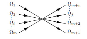
In this paper we consider a scalar parabolic equation on a star graph; the model is quite general but what we have in mind is the description of traffic flows at a crossroad. In particular, we do not necessarily require the continuity of the unknown function at the node of the graph and, moreover, the diffusivity can be degenerate. Our main result concerns a necessary and sufficient algebraic condition for the existence of traveling waves in the graph. We also study in great detail some examples corresponding to quadratic and logarithmic flux functions, for different diffusivities, to which our results apply.
Citation: Andrea Corli, Lorenzo di Ruvo, Luisa Malaguti, Massimiliano D. Rosini. Traveling waves for degenerate diffusive equations on networks[J]. Networks and Heterogeneous Media, 2017, 12(3): 339-370. doi: 10.3934/nhm.2017015
In this paper we consider a scalar parabolic equation on a star graph; the model is quite general but what we have in mind is the description of traffic flows at a crossroad. In particular, we do not necessarily require the continuity of the unknown function at the node of the graph and, moreover, the diffusivity can be degenerate. Our main result concerns a necessary and sufficient algebraic condition for the existence of traveling waves in the graph. We also study in great detail some examples corresponding to quadratic and logarithmic flux functions, for different diffusivities, to which our results apply.

| [1] | A. Ambroso, C. Chalons, F. Coquel, E. Godlewski, F. Lagoutière, P. -A. Raviart and N. Seguin, The coupling problem of different thermal-hydraulic models arising in two-phase flow codes for nuclear reactors, in Coupled Problems, CIMNE, Barcelona, (2009), 1–5. |
| [2] |
Flows on networks: Recent results and perspectives. EMS Surv. Math. Sci. (2014) 1: 47-111. 
|
| [3] |
Non-local first-order modelling of crowd dynamics: A multidimensional framework with applications. Appl. Math. Model. (2011) 35: 426-445.
|
| [4] |
Vanishing viscosity for traffic on networks. SIAM J. Math. Anal. (2010) 42: 1761-1783.
|
| [5] |
Traffic flow on a road network. SIAM J. Math. Anal. (2005) 36: 1862-1886.
|
| [6] |
A. Corli, L. di Ruvo and L. Malaguti, Sharp profiles in models of collective movements Nonlinear Diff. Equat. Appl. NoDEA, 24 (2017), p24. doi: 10.1007/s00030-017-0460-z
|
| [7] |
Semi-wavefront solutions in models of collective movements with density-dependent diffusivity. Dyn. Partial Differ. Equ. (2016) 13: 297-331.
|
| [8] |
R. Dáger and E. Zuazua, Wave Propagation, Observation and Control in 1-d Flexible Multi-Structures volume 50 of Mathématiques & Applications (Berlin) [Mathematics & Applications], Springer-Verlag, Berlin, 2006. doi: 10.1007/3-540-37726-3
|
| [9] |
M. R. Flynn, A. R. Kasimov, J. -C. Nave, R. R. Rosales and B. Seibold, Self-sustained nonlinear waves in traffic flow,
Phys. Rev. E (3), 79 (2009), 056113, 13pp. doi: 10.1103/PhysRevE.79.056113
|
| [10] | M. Garavello, K. Han and B. Piccoli, Models for Vehicular Traffic on Networks, volume 9 of AIMS Series on Applied Mathematics, American Institute of Mathematical Sciences (AIMS), Springfield, MO, 2016. |
| [11] | M. Garavello and B. Piccoli, Traffic Flow on Networks, volume 1 of AIMS Series on Applied Mathematics, American Institute of Mathematical Sciences (AIMS), Springfield, MO, 2006. |
| [12] |
B. H. Gilding and R. Kersner,
Travelling Waves in Nonlinear Diffusion-Convection Reaction, Birkhäuser Verlag, Basel, 2004. doi: 10.1007/978-3-0348-7964-4
|
| [13] |
An analysis of traffic flow. Operations Research (1959) 7: 79-85.
|
| [14] | A study of traffic capacity. Proceedings of the Highway Research Board (1935) 14: 448-477. |
| [15] |
Traffic and related self-driven many-particle systems. Rev. Mod. Phys. (2001) 73: 1067-1141.
|
| [16] |
J. E. Lagnese, G. Leugering and E. J. P. G. Schmidt,
Modeling, Analysis and Control of Dynamic Elastic Multi-Link Structures, Systems & Control: Foundations & Applications. Birkhäuser Boston, Inc. , Boston, MA, 1994. doi: 10.1007/978-1-4612-0273-8
|
| [17] |
On kinematic waves. Ⅱ. A theory of traffic flow on long crowded roads. Proc. Roy. Soc. London. Ser. A. (1955) 229: 317-345.
|
| [18] |
D. Mugnolo,
Semigroup Methods for Evolution Equations on Networks, Springer, Cham, 2014. doi: 10.1007/978-3-319-04621-1
|
| [19] | Construction of exact travelling waves for the {B}enjamin-{B}ona-{M}ahony equation on networks. Bull. Belg. Math. Soc. Simon Stevin (2014) 21: 415-436. |
| [20] | Synchronized traffic flow from a modified Lighthill-Whitham model. Phys. Review E (2000) 61: R6052-R6055. |
| [21] |
Traveling-wave solutions of the diffusively corrected kinematic-wave model. Math. Comput. Modelling (2002) 35: 561-579.
|
| [22] | Models of freeway traffic and control. Simulation Council Proc. (1971) 1: 51-61. |
| [23] |
Car following models and the fundamental diagram of road traffic. Transp. Res. (1967) 1: 21-29.
|
| [24] |
Differential equations on networks (geometric graphs). J. Math. Sci. (N. Y.) (2004) 119: 691-718.
|
| [25] |
Shock waves on the highway. Oper. Res. (1956) 4: 42-51.
|
| [26] |
M. D. Rosini,
Macroscopic Models for Vehicular Flows and Crowd Dynamics: Theory and Applications, Springer, Heidelberg, 2013. doi: 10.1007/978-3-319-00155-5
|
| [27] | Empirical features of congested traffic states and their implications for traffic modeling. Transportation Science (2007) 41: 135-166. |
| [28] |
Constructing set-valued fundamental diagrams from jamiton solutions in second order traffic models. Netw. Heterog. Media (2013) 8: 745-772.
|
| [29] |
Classical solvability of linear parabolic equations on networks. J. Differential Equations (1988) 72: 316-337.
|
| [30] | J. von Below, Parabolic Network Equations, Ph. D thesis, Tübinger Universitätsverlag, Tübingen, 1994. |
| [31] | J. von Below, Front propagation in diffusion problems on trees, in Calculus of Variations, Applications and Computations, Pitman Res. Notes Math. Ser. , 326, Longman Sci. Tech. , Harlow, 1995,254–265. |


Figures(4)
Andrea Corli, Lorenzo di Ruvo, Luisa Malaguti, Massimiliano D. Rosini. Traveling waves for degenerate diffusive equations on networks[J]. Networks and Heterogeneous Media, 2017, 12(3): 339-370. doi: 10.3934/nhm.2017015


 DownLoad: