Investigation of biocorrosion on mild steel in cooling tower water and its inhibition by <i>C. sativum</i>

Sharmil Suganya R; Stanelybritto Maria Arul Francis; T Venugopal; Sharmil Suganya R; Stanelybritto Maria Arul Francis; T Venugopal

doi:10.3934/molsci.2024024

AIMS Molecular Science

2024, Volume 11, Issue 4: 395-414. doi: 10.3934/molsci.2024024

Previous Article Next Article

Research article

Investigation of biocorrosion on mild steel in cooling tower water and its inhibition by C. sativum

Government College of Engineering, Salem-11, Tamil Nadu, India

Received: 28 July 2024 Revised: 16 November 2024 Accepted: 25 November 2024 Published: 18 December 2024

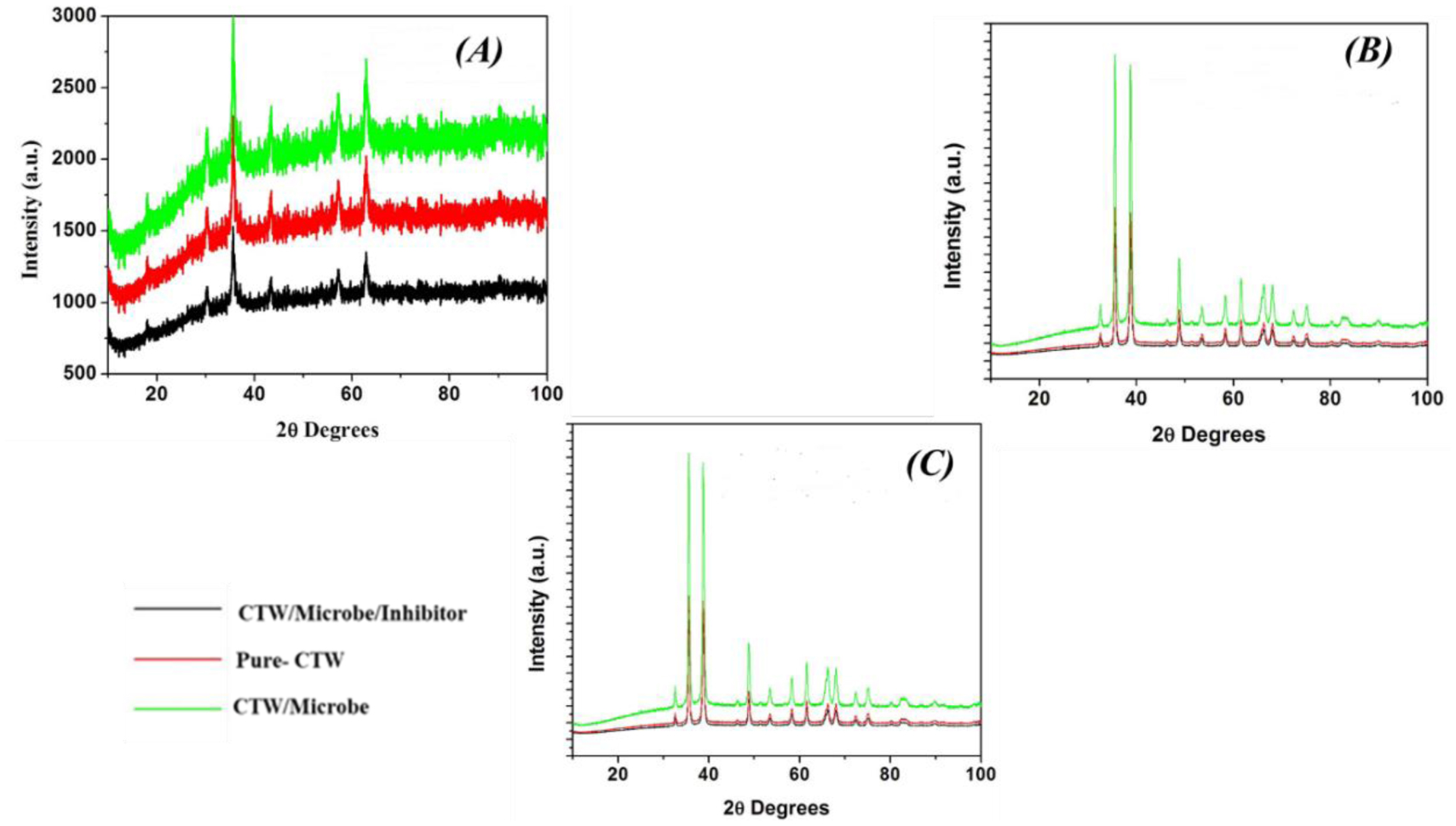
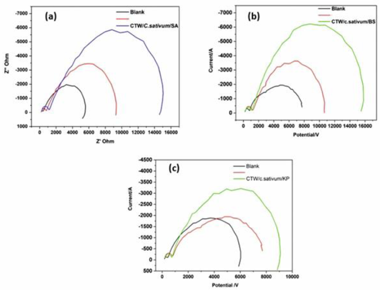
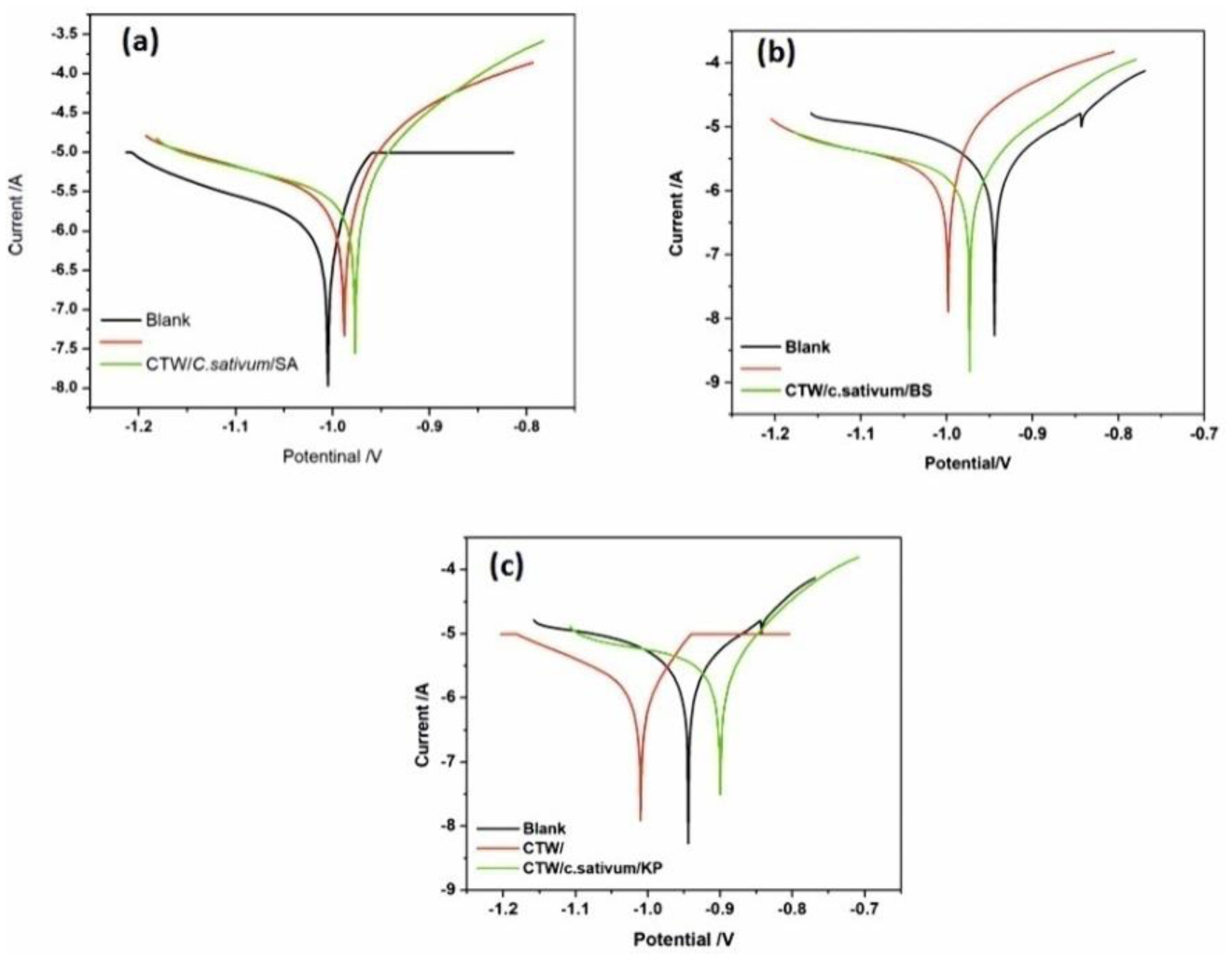
The primary goal of this investigation was to evaluate the effect of Coriandrum sativum extract on mitigating corrosion caused by Staphylococcus aureus, Klebsiella pneumonia, and Bacillus subtilis on metal samples. Analytical methods including SEM, FTIR, and XRD examination were used on the metal surface to determine the mechanism underlying corrosion inhibition. Impedance studies and Nyquist plots were used to support the role of green inhibitors in biocorrosion control. Based on analytical examinations, the corrosion patterns in some pitted zones showed a substantial link between microbial metabolites and the chemical composition of the metal surface. The presence of microbial metabolites caused the metallic surface to become more porous and permeable, changing the surface's structural makeup. In all three bacteria, 30 ppm of plant extract was found to be the maximum concentration that inhibited microbial corrosion. The coupons submerged in the control solution lost weight, indicating that the addition of the inhibitor caused a brief increase in corrosion rates before they declined.
- microbial-induced corrosion,
- biofilm,
- plant extracts,
- Nyquist plots,
- SEM,
- FTIR
Citation: Sharmil Suganya R, Stanelybritto Maria Arul Francis, T Venugopal. Investigation of biocorrosion on mild steel in cooling tower water and its inhibition by C. sativum[J]. AIMS Molecular Science, 2024, 11(4): 395-414. doi: 10.3934/molsci.2024024

Related Papers:

Abstract

The primary goal of this investigation was to evaluate the effect of Coriandrum sativum extract on mitigating corrosion caused by Staphylococcus aureus, Klebsiella pneumonia, and Bacillus subtilis on metal samples. Analytical methods including SEM, FTIR, and XRD examination were used on the metal surface to determine the mechanism underlying corrosion inhibition. Impedance studies and Nyquist plots were used to support the role of green inhibitors in biocorrosion control. Based on analytical examinations, the corrosion patterns in some pitted zones showed a substantial link between microbial metabolites and the chemical composition of the metal surface. The presence of microbial metabolites caused the metallic surface to become more porous and permeable, changing the surface's structural makeup. In all three bacteria, 30 ppm of plant extract was found to be the maximum concentration that inhibited microbial corrosion. The coupons submerged in the control solution lost weight, indicating that the addition of the inhibitor caused a brief increase in corrosion rates before they declined.

Acknowledgments

We are quite grateful to the Government College of Engineering, Salem, for funding and providing facilities for the study and providing us with the opportunity to successfully finish our research project. We would like to express our gratitude to the Department of Chemistry Laboratory's scientific team for their important support during the experimental investigation.

Conflict of interest

The authors declare that there is no conflict of interest.

References

[1]	Hamak KF (2014) Synthesis of phthalimides via the reaction of phthalic anhydride with amines & evaluating of its biological & anti-corrosion activity. Int J Chem Tech Res 6: 324-333.
[2]	El-Shanshoury AER, ElSilk S, Ebeid ME (2011) Extracellular biosynthesis of silver nanoparticles using Escherichia coli ATCC 8739, Bacillus subtilis ATCC 6633, and Streptococcus thermophilus ESh1 and their antimicrobial activities. Int Scholarly Res Notices 2011: 385480. https://doi.org/10.5402/2011/385480
[3]	Sahib NG, Anwar F, Gilani AH, et al. (2012) Coriander (Coriandrum sativum L.): A potential source of high-value components for functional foods and nutraceuticals-A review. Phytother Res 27: 1439-1456. https://doi.org/10.1002/ptr.4897
[4]	Kubo I, Fujita KI, Kubo A, et al. (2004) Antibacterial activity of coriander volatile compounds against Salmonella cholerasuis. J Agric Food Chem 52: 3329-3332. https://doi.org/10.1021/jf0354186
[5]	Saeed S, Tariq P (2007) Antimicrobial activities of Emblica officinalis and Coriandrum sativum against Gram-positive bacteria and Candida albicans. Pak J Bot 39: 913-917.
[6]	Begnami AF, Duarte MCT, Furletti V, et al. (2010) Antimicrobial potential of Coriandrum sativum L. against different Candida species in vitro. Food Chem 118: 74-77. https://doi.org/10.1016/j.foodchem.2009.04.089
[7]	Al-Snafi AE (2016) A review on chemical constituents and pharmacological activities of Coriandrum sativum. IOSR J Pharm 6: 17-42. https://doi.org/10.9790/3013-067031742
[8]	Sastri BN (1950) Coriandrum sativum Linn (Umbelliferae). The wealth of India: A dictionary of Indian raw materials and industrial products (Vol 2). New Delhi: Council of Scientific and Industrial Research 347-350.
[9]	WFOCoriandrum sativum L (2024). Available from: http://www.worldfloraonline.org/tpl/kew-2737546
[10]	Da Rocha Magalhães L, da Silva Alvarenga RF, Resende FAC, et al. (2023) The synergy between corrosion and fatigue: Failure analysis of an aerator and a cooling tower. J Fail Anal Prev 23: 1803-1819. https://doi.org/10.1007/s11668-023-01729-1
[11]	Kokilaramani S, Al-Ansari MM, Rajasekar A, et al. (2021) Microbial influenced corrosion of processing industry by re-circulating wastewater and its control measures—A review. Chemosphere 265: 129075. https://doi.org/10.1016/j.chemosphere.2020.129075
[12]	Telegdi J, Shaban A, Trif L (2017) Microbiologically influenced corrosion (MIC). Trends in oil and gas corrosion research and technologies : 191-214. https://doi.org/10.1016/B978-0-08-101105-8.00008-5
[13]	Kuraimid ZK, Majeed HM, Jebur HQ, et al. (2021) Synthesis of new corrosion inhibitors with high efficiency in aqueous and oil phase for low carbon steel for Missan oil field equipment. Eurasian Chem Commun 3: 860-871. https://doi.org/10.22034/ecc.2021.302887.1233
[14]	Kaya F, Solmaz R, Gecibesler IH (2023) Adsorption and corrosion inhibition capability ofRheum ribesroot extract (Işgın) for mild steel protection in acidic medium: A comprehensive electrochemical, surface characterization, synergistic inhibition effect, and stability study. J Mol Liq 372: 121219. https://doi.org/10.1016/j.molliq.2023.121219
[15]	Hossain SMZ, Razzak SA, Hossain MM (2020) Application of essential oils as green corrosion inhibitors. Arab J Sci Eng 45: 7137-7159. https://doi.org/10.1007/s13369-019-04305-8
[16]	Sezonov G, Joseleau-Petit D, D'Ari R (2007) Escherichia coli physiology in Luria-Bertani broth. J Bacteriol 189: 8746-8749. https://doi.org/10.1128/JB.01368-07
[17]	Balouiri M, Sadiki M, Ibnsouda SK (2016) Methods for in vitro evaluating antimicrobial activity: A review. J Pharm Anal 6: 71-79. https://doi.org/10.1016/j.jpha.2015.11.005
[18]	Narenkumar J, Parthipan P, Nanthini AUR, et al. (2017) Ginger extract as green biocide to control microbial corrosion of mild steel. 3 Biotech 7: 133. https://doi.org/10.1007/s13205-017-0783-9
[19]	Rajasekar V, Shyamala M, Aravind J (2024) Green, environmentally friendly synthesis of MnO nanoparticles for corrosion inhibition in mild steel. Glob NEST J 26: 1-12. https://doi.org/10.30955/gnj.05891
[20]	Nwigwe US, Mbam SO, Umunakwe R (2019) Evaluation of Carica papaya leaf extract as a bio-corrosion inhibitor for mild steel applications in a marine environment. Mater Res Express 6: 105107. https://doi.org/10.1088/2053-1591/ab3ff6
[21]	Agarry SE, Oghenejoboh KM, Aworanti OA, et al. (2019) Biocorrosion inhibition of mild steel in crude oil-water environment using extracts of Musa paradisiaca peels, Moringa oleifera leaves, and Carica papaya peels as biocidal-green inhibitors: Kinetics and adsorption studies. Chem Eng Commun 206: 98-124. https://doi.org/10.1080/00986445.2018.1476855
[22]	Karunanithi A, Venkatachalam S (2019) Ultrasonic-assisted solvent extraction of phenolic compounds from Opuntia ficus-indica peel: Phytochemical identification and comparison with Soxhlet extraction. J Food Process Eng 42: e13126. https://doi.org/10.1111/jfpe.13126
[23]	Pal MK, Lavanya M (2022) Microbial influenced corrosion: Understanding bioadhesion and biofilm formation. J Bio TriboCorros 8: 76. https://doi.org/10.1007/s40735-022-00677-x
[24]	Loto CA (2017) Microbiological corrosion: Mechanism, control, and impact—A review. Int J Adv Manuf Technol 92: 4241-4252. https://doi.org/10.1007/s00170-017-0494-8
[25]	Knisz J, Eckert R, Gieg LM, et al. (2023) Microbiologically influenced corrosion—more than just microorganisms. FEMS Microbiol Rev 47: fuad041. https://doi.org/10.1093/femsre/fuad041
[26]	Molina RDI, Campos-Silva R, Macedo AJ, et al. (2020) Antibiofilm activity of coriander (Coriander sativum L.) grown in Argentina against food contaminants and human pathogenic bacteria. Ind Crops Prod 151: 112380. https://doi.org/10.1016/j.indcrop.2020.112380
[27]	Lin Q, Li Y, Sheng M, et al. (2023) Antibiofilm effects of berberine-loaded chitosan nanoparticles against Candida albicans biofilm. LWT 173: 114237. https://doi.org/10.1016/j.lwt.2022.114237
[28]	da Silva BD, Bernardes PC, Pinheiro PF, et al. (2021) Chemical composition, extraction sources, and action mechanisms of essential oils: Natural preservative and limitations of use in meat products. Meat Sci 176: 108463. https://doi.org/10.1016/j.meatsci.2021.108463
[29]	Caldwell DE, Korber DR, Lawrence LR (1992) Confocal laser microscopy and digital image analysis in microbial ecology. Advances in microbial ecology. Boston, MA: Springer 1-67. https://doi.org/10.1007/978-1-4684-7609-5_1
[30]	Mohd Ali MKFB, Abu Bakar A, Noor NM, et al. (2017) Hybrid soliwave technique for mitigating sulfate-reducing bacteria in controlling biocorrosion: A case study on crude oil sample. Environ Technol 38: 2427-2439. https://doi.org/10.1080/09593330.2016.1264486
[31]	Albahri MB, Barifcani A, Iglauer S, et al. (2021) Investigating the mechanism of microbiologically influenced corrosion of carbon steel using X-ray micro-computed tomography. J Mater Sci 56: 13337-13371. https://doi.org/10.1007/s10853-021-06112-9
[32]	Malek TJ, Chaki SH, Deshpande MP (2018) Structural, morphological, optical, thermal and magnetic study of mackinawite FeS nanoparticles synthesized by wet chemical reduction technique. Physica B 546: 59-66. https://doi.org/10.1016/j.physb.2018.07.024
[33]	Otton LM, da Silva Campos M, Meneghetti KL, et al. (2017) Influence of twitching and swarming motilities on biofilm formation in Pseudomonas strains. Arch Microbiol 199: 677-682. https://doi.org/10.1007/s00203-017-1344-7
[34]	Karthik R, Muthukrishnan P, Chen SM, et al. (2015) Anti-corrosion inhibition of mild steel in 1M hydrochloric acid solution by using Tiliacora accuminata leaves extract. Int J Electrochem Sci 10: 3707-3725. https://doi.org/10.1016/S1452-3981(23)06573-2
[35]	AlSalhi MS, Devanesan S, Rajasekar A, et al. (2023) Characterization of plants and seaweeds based corrosion inhibitors against microbially influenced corrosion in a cooling tower water environment. Arab J Chem 16: 104513. https://doi.org/10.1016/j.arabjc.2022.104513
[36]	Sourmaghi MH, Kiaee G, Golfakhrabadi F, et al. (2015) Comparison of essential oil composition and antimicrobial activity of Coriandrum sativum L. extracted by hydrodistillation and microwave-assisted hydrodistillation. J Food Sci Technol 52: 2452-2457. https://doi.org/10.1007/s13197-014-1286-x
[37]	Murungi PI, Sulaimon AA (2022) Ideal corrosion inhibitors: A review of plant extracts as corrosion inhibitors for metal surfaces. Corros Rev 40: 127-136. https://doi.org/10.1515/corrrev-2021-0051
[38]	Videla HA (1996) Manual of biocorrosion. New York: Routledge. https://doi.org/10.1201/9780203748190
[39]	Ech-chihbi E, Adardour M, Ettahiri W, et al. (2023) Surface interactions and improved corrosion resistance of mild steel by addition of new triazolyl-benzimidazolone derivatives in acidic environment. J Mol Liq 387: 122652. https://doi.org/10.1016/j.molliq.2023.122652
[40]	Cai T, Zhang Y, Wang N, et al. (2022) Electrochemically active microorganisms sense charge transfer resistance for regulating biofilm electroactivity, spatio-temporal distribution, and catabolic pathway. Chem Eng J 442: 136248. https://doi.org/10.1016/j.cej.2022.136248
[41]	Pais M, Rao P (2021) Electrochemical, spectroscopic and theoretical studies for acid corrosion of zinc using glycogen. Chem Pap 75: 1387-1399. https://doi.org/10.1007/s11696-020-01391-z
[42]	Xu D, Li Y, Gu T (2016) Mechanistic modelling of biocorrosion caused by biofilms of sulfate reducing bacteria and acid producing bacteria. Bioelectrochemistry 110: 52-58. https://doi.org/10.1016/j.bioelechem.2016.03.003
[43]	Karn SK, Fang G, Duan J (2017) Bacillus sp. acting as dual role for corrosion induction and corrosion inhibition with carbon steel (CS). Front Microbiol 8: 02038. https://doi.org/10.3389/fmicb.2017.02038
[44]	Farh HMH, Ben Seghier MEA, Zayed T (2023) A comprehensive review of corrosion protection and control techniques for metallic pipelines. Eng Fail Anal 143: 106885. https://doi.org/10.1016/j.engfailanal.2022.106885
[45]	Kumari PP, Shetty P, Rao SA (2017) Electrochemical measurements for the corrosion inhibition of mild steel in 1M hydrochloric acid by using an aromatic hydrazide derivative. Arab J Chem 10: 653-663. https://doi.org/10.1016/j.arabjc.2014.09.005
[46]	Narenkumar J, Parthipan P, Madhavan J, et al. (2018) Bioengineered silver nanoparticles as potent anti-corrosive inhibitor for mild steel in cooling towers. Environ Sci Pollut Res 25: 5412-5420. https://doi.org/10.1007/s11356-017-0768-6
[47]	Permeh S, Lau K, Duncan M (2019) Characterization of biofilm formation and coating degradation by electrochemical impedance spectroscopy. Coatings 9: 518. https://doi.org/10.3390/coatings9080518
[48]	Fojt J, Průchová E, Hybášek V (2023) Electrochemical impedance response of the nanostructured Ti–6Al–4V surface in the presence of S. aureus and E. coli. J Appl Electrochem 53: 2153-2167. https://doi.org/10.1007/s10800-023-01911-1
[49]	Kim T, Kang J, Lee JH, et al. (2011) Influence of attached bacteria and biofilm on double-layer capacitance during biofilm monitoring by electrochemical impedance spectroscopy. Water Res 45: 4615-4622. https://doi.org/10.1016/j.watres.2011.06.010
[50]	Victoria SN, Sharma A, Manivannan R (2021) Metal corrosion induced by microbial activity–Mechanism and control options. J Indian Chem Soc 98: 100083. https://doi.org/10.1016/j.jics.2021.100083
[51]	Caldona EB, de Leon ACC, Mangadlao JD, et al. (2018) On the enhanced corrosion resistance of elastomer-modified polybenzoxazine/graphene oxide nanocomposite coatings. React Funct Polym 123: 10-19. https://doi.org/10.1016/j.reactfunctpolym.2017.12.004
[52]	Olasunkanmi LO, Obot IB, Kabanda MM, et al. (2015) Some quinoxalin-6-yl derivatives as corrosion inhibitors for mild steel in hydrochloric acid: Experimental and theoretical studies. J Phys Chem C 119: 16004-16019. https://doi.org/10.1021/acs.jpcc.5b03285
[53]	Rao P, Mulky L (2023) Microbially influenced corrosion and its control measures: A critical review. J Bio Tribo Corros 9: 57. https://doi.org/10.1007/s40735-023-00772-7
[54]	Briggs WF, Stanley HO, Okpokwasili GC, et al. (2019) Biocorrosion inhibitory potential of aqueous extract of Phyllanthus amarus against acid-producing bacteria. J Adv Biol Biotechnol 22: 1-8. https://doi.org/10.9734/jabb/2019/v22i130106

Reader Comments

Your name:*

Email:*
© 2024 the Author(s), licensee AIMS Press. This is an open access article distributed under the terms of the Creative Commons Attribution License (http://creativecommons.org/licenses/by/4.0)