Toward autism spectrum disorders and Williams-Beuren syndrome co-occurrence condition in Tunisian patients: Genetic insights

Rim Khelifi; Afef Jelloul; Houda Ajmi; Wafa Slimani; Sarra Dimassi; Khouloud Rjiba; Manel Dardour; Moez Gribaa; Ali Saad; Soumaya Mougou-Zerelli; Rim Khelifi; Afef Jelloul; Houda Ajmi; Wafa Slimani; Sarra Dimassi; Khouloud Rjiba; Manel Dardour; Moez Gribaa; Ali Saad; Soumaya Mougou-Zerelli

doi:10.3934/molsci.2024023

AIMS Molecular Science

2024, Volume 11, Issue 4: 379-394. doi: 10.3934/molsci.2024023

Previous Article Next Article

Research article

Toward autism spectrum disorders and Williams-Beuren syndrome co-occurrence condition in Tunisian patients: Genetic insights

1.
Laboratory of Cytogenetics, Molecular Genetics and Human Reproductive Biology CHU Farhat Hached Sousse, Tunisia
2.
Common Service Unit in Genetics, Faculty of Medicine Sousse, Tunisia
3.
Higher Institute of Biotechnology Monastir, Monastir University, Tunisia
4.
Pasteur institute Tunis, Tunisia
5.
Paediatric Department, Sahloul University Hospital Sousse, Tunisia
6.
Pedopsychiatrist, private practice Sousse, Tunisia

Received: 20 July 2024 Revised: 25 October 2024 Accepted: 07 November 2024 Published: 29 November 2024

Introduction
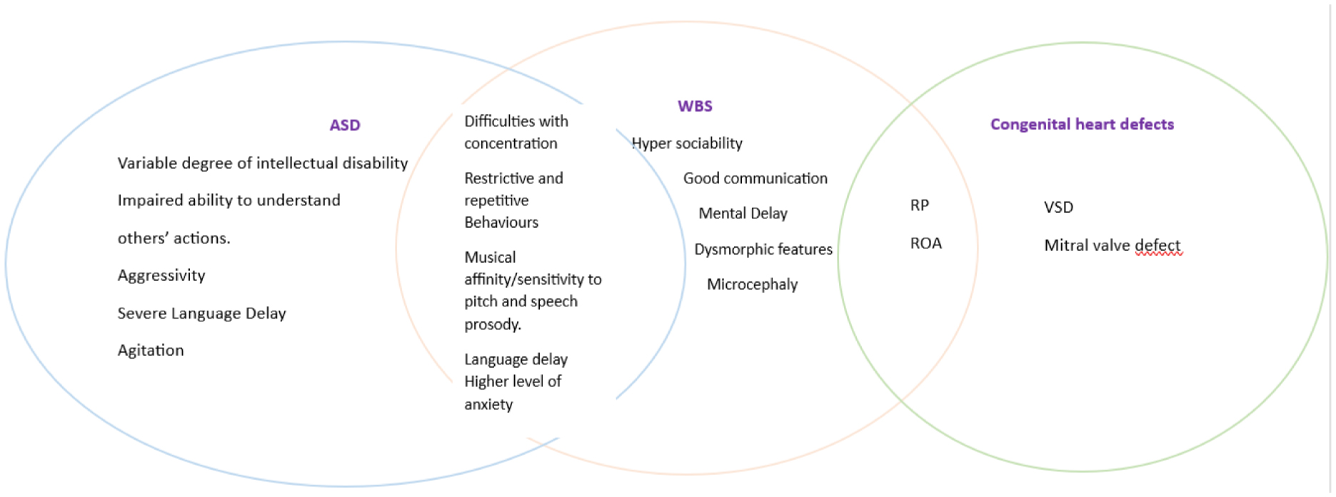
Williams-Beuren syndrome (WBS) is a rare genetic disorder characterized by congenital heart defects, dysmorphic features, intellectual delay, and a distinctive social behavioral profile. This highly recurrent and homogeneous phenotype has been curiously reported to be associated with autism spectrum disorders (ASD). Both genetic and environmental origins have been implicated. This study aimed to describe Tunisian patients associated with WBS and ASD and explore the underlying etiologies.
Methods
Thirty-one clinically suspected WBS were referred for genetic exploration. A comprehensive evaluation using karyotyping, fluorescence in situ hybridization (FISH), and array comparative genomic hybridization (array-CGH) was performed.
Results
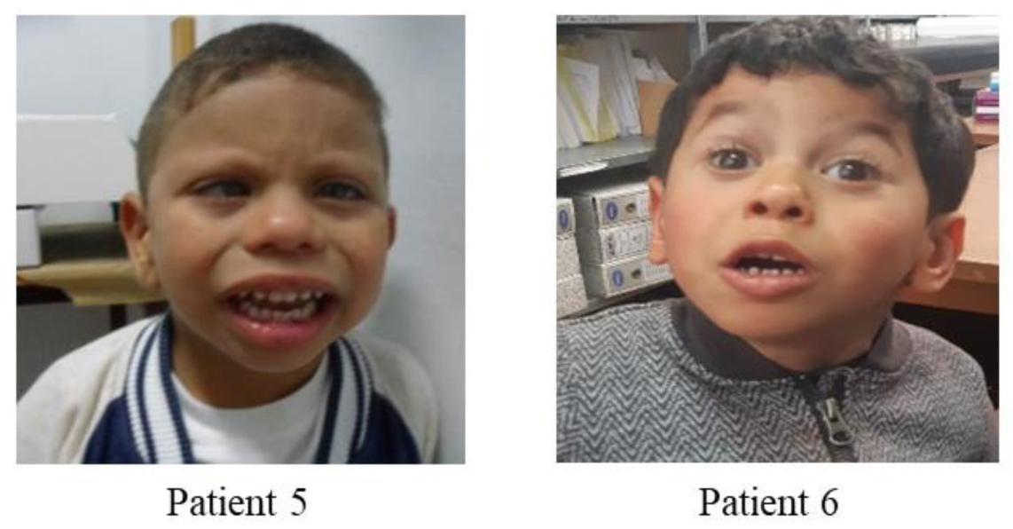
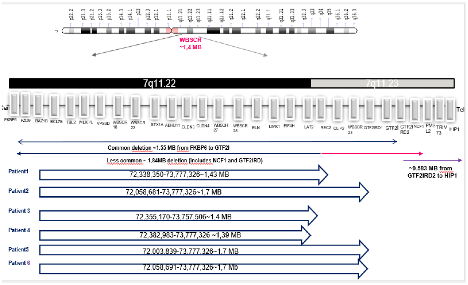
All patients were clinically diagnosed and confirmed to have WBS through karyotyping and FISH analysis. Notably, six patients with complex or atypical clinical presentations underwent array-CGH. Two of these patients presented with ASD. Array CGH showed microdeletions ranging from 1.4 to 1.7 Mb in the 7q11.2 region. Further analysis of the extended region deletion identified a gene closely located in the deleted region, the HIP1 gene, involved in the central nervous system trafficking protein.
Discussion
The recurrent deletion in WBS, as well as the mirror duplication, may contribute to ASD development in some cases, suggesting a potential involvement of the ASD genes pathway in this region. However, recessive genetic origins should also be considered, particularly in consanguineous families. Furthermore, our findings highlight the potential role of genetic factors and regulatory elements within the deleted region in modulating gene expression, notably the HIP1 gene. This underscores the implications of gene dosage and environmental factors in the broader WBS region, notably with language and social development.
Conclusion
The presence of ASD in WBS patients emphasizes the need to investigate all WBS patients for autistic traits to establish a better genotype–phenotype correlation. We underline the utility of array-CGH as a valuable genetic diagnostic tool for characterizing WBS cases, and we shed light on the complex interplay of behavioral disorders in the 7q11.2 region rearrangements.
- CGH-array,
- Williams Beuren-syndrome,
- autistic traits,
- HIP1
Citation: Rim Khelifi, Afef Jelloul, Houda Ajmi, Wafa Slimani, Sarra Dimassi, Khouloud Rjiba, Manel Dardour, Moez Gribaa, Ali Saad, Soumaya Mougou-Zerelli. Toward autism spectrum disorders and Williams-Beuren syndrome co-occurrence condition in Tunisian patients: Genetic insights[J]. AIMS Molecular Science, 2024, 11(4): 379-394. doi: 10.3934/molsci.2024023

Related Papers:

Abstract

Introduction

Williams-Beuren syndrome (WBS) is a rare genetic disorder characterized by congenital heart defects, dysmorphic features, intellectual delay, and a distinctive social behavioral profile. This highly recurrent and homogeneous phenotype has been curiously reported to be associated with autism spectrum disorders (ASD). Both genetic and environmental origins have been implicated. This study aimed to describe Tunisian patients associated with WBS and ASD and explore the underlying etiologies.

Methods

Thirty-one clinically suspected WBS were referred for genetic exploration. A comprehensive evaluation using karyotyping, fluorescence in situ hybridization (FISH), and array comparative genomic hybridization (array-CGH) was performed.

Results

All patients were clinically diagnosed and confirmed to have WBS through karyotyping and FISH analysis. Notably, six patients with complex or atypical clinical presentations underwent array-CGH. Two of these patients presented with ASD. Array CGH showed microdeletions ranging from 1.4 to 1.7 Mb in the 7q11.2 region. Further analysis of the extended region deletion identified a gene closely located in the deleted region, the HIP1 gene, involved in the central nervous system trafficking protein.

Discussion

The recurrent deletion in WBS, as well as the mirror duplication, may contribute to ASD development in some cases, suggesting a potential involvement of the ASD genes pathway in this region. However, recessive genetic origins should also be considered, particularly in consanguineous families. Furthermore, our findings highlight the potential role of genetic factors and regulatory elements within the deleted region in modulating gene expression, notably the HIP1 gene. This underscores the implications of gene dosage and environmental factors in the broader WBS region, notably with language and social development.

Conclusion

The presence of ASD in WBS patients emphasizes the need to investigate all WBS patients for autistic traits to establish a better genotype–phenotype correlation. We underline the utility of array-CGH as a valuable genetic diagnostic tool for characterizing WBS cases, and we shed light on the complex interplay of behavioral disorders in the 7q11.2 region rearrangements.

Acknowledgments

We are very grateful to the family members for their kind participation and their continuous interest in this study. We also thank the scientific and technical team of the cytogenetics Department at Farhat Hached University Teaching Hospital (Sousse, Tunisia).

Conflict of interest

All authors declare no conflicts of interest in this paper.

References

[1]	Ramírez-Velazco A, Aguayo-Orozco TA, Figuera L, et al. (2019) Williams–Beuren syndrome in Mexican patients confirmed by FISH and assessed by aCGH. J Genet 98: 34. https://doi.org/10.1007/s12041-019-1080-7
[2]	Yuan SM (2017) Congenital heart defects in Williams syndrome. Turk J Pediatr 59: 225-231. https://doi.org/10.24953/turkjped.2017.03.001
[3]	Debelle L, Tamburro AM (1999) Elastin: Molecular description and function. Int J Biochem Cell Biol 31: 261-272. https://doi.org/10.1016/S1357-2725(98)00098-3
[4]	Ewart AK, Morris CA, Atkinson D, et al. (1993) Hemizygosity at the elastin locus in a developmental disorder, Williams syndrome. Nat Genet 5: 11-16. https://doi.org/10.1038/ng0993-11
[5]	van der Bom T, Zomer AC, Zwinderman AH, et al. (2011) The changing epidemiology of congenital heart disease. Nat Rev Cardiol 8: 50-60. https://doi.org/10.1038/nrcardio.2010.166
[6]	Schopler E, Reichler RJ, DeVellis RF, et al. (1980) Toward objective classification of childhood autism: Childhood Autism Rating Scale (CARS). J Autism Dev Disord 10: 91-103. https://doi.org/10.1007/BF02408436
[7]	Edelmann L, Prosnitz A, Pardo S, et al. (2006) An atypical deletion of the Williams-Beuren syndrome interval implicates genes associated with defective visuospatial processing and autism. J Med Genet 44: 136-143. https://doi.org/10.1136/jmg.2006.044537
[8]	Depienne C, Heron D, Betancur C, et al. (2007) Autism, language delay and mental retardation in a patient with 7q11 duplication. J Med Genet 44: 452-458. https://doi.org/10.1136/jmg.2006.047092
[9]	Berg JS, Brunetti-Pierri N, Peters SU, et al. (2007) Speech delay and autism spectrum behaviors are frequently associated with duplication of the 7q11.23 Williams-Beuren syndrome region. Genet Med 9: 427-441. https://doi.org/10.1097/GIM.0b013e3180986192
[10]	Fusco C, Micale L, Augello B, et al. (2014) Smaller and larger deletions of the Williams Beuren syndrome region implicate genes involved in mild facial phenotype, epilepsy and autistic traits. Eur J Hum Genet 22: 64-70. https://doi.org/10.1038/ejhg.2013.101
[11]	Alesi V, Loddo S, Orlando V, et al. (2021) Atypical 7q11.23 deletions excluding ELN gene result in Williams–Beuren syndrome craniofacial features and neurocognitive profile. Am J Med Genet A 185: 242-249. https://doi.org/10.1002/ajmg.a.61937
[12]	Kruszka P, Porras AR, de Souza DH, et al. (2018) Williams–Beuren syndrome in diverse populations. Am J Med Genet A 176: 1128-1136. https://doi.org/10.1002/ajmg.a.38672
[13]	Lee CL, Lin SM, Chen MR, et al. (2022) Long-term cardiovascular findings in Williams syndrome: A single medical center experience in Taiwan. J Pers Med 12: 817. https://doi.org/10.3390/jpm12050817
[14]	Niego A, Benítez-Burraco A (2022) Autism and Williams syndrome: truly mirror conditions in the socio-cognitive domain?. Int J Dev Disabil 68: 399-415. https://doi.org/10.1080/20473869.2020.1817717
[15]	Richards C, Jones C, Groves L, et al. (2015) Prevalence of autism spectrum disorder phenomenology in genetic disorders: a systematic review and meta-analysis. Lancet Psychiat 2: 909-916. https://doi.org/10.1016/S2215-0366(15)00376-4
[16]	Masson J, Demily C, Chatron N, et al. (2019) Molecular investigation, using chromosomal microarray and whole exome sequencing, of six patients affected by Williams Beuren syndrome and Autism Spectrum Disorder. Orphanet J Rare Dis 14: 121. https://doi.org/10.1186/s13023-019-1094-5
[17]	Ramocki MB, Bartnik M, Szafranski P, et al. (2010) Recurrent distal 7q11.23 deletion including HIP1 and YWHAG identified in patients with intellectual disabilities, epilepsy, and neurobehavioral problems. Am J Hum Genet 87: 857-865. https://doi.org/10.1016/j.ajhg.2010.10.019
[18]	Sanders SJ, Ercan-Sencicek AG, Hus V, et al. (2011) Multiple recurrent de novo CNVs, including duplications of the 7q11.23 Williams syndrome region, are strongly associated with autism. Neuron 70: 863-885. https://doi.org/10.1016/j.neuron.2011.05.002

Reader Comments

Your name:*

Email:*
© 2024 the Author(s), licensee AIMS Press. This is an open access article distributed under the terms of the Creative Commons Attribution License (http://creativecommons.org/licenses/by/4.0)