
Citation: Larisa I. Fedoreyeva, Boris F. Vanyushin. Possible existence of a system similar to bacterial restriction–modification in plants[J]. AIMS Molecular Science, 2020, 7(4): 396-413. doi: 10.3934/molsci.2020020
[1] | Muhammad Asim Khan, Norma Alias, Umair Ali . A new fourth-order grouping iterative method for the time fractional sub-diffusion equation having a weak singularity at initial time. AIMS Mathematics, 2023, 8(6): 13725-13746. doi: 10.3934/math.2023697 |
[2] | Mubashara Wali, Sadia Arshad, Sayed M Eldin, Imran Siddique . Numerical approximation of Atangana-Baleanu Caputo derivative for space-time fractional diffusion equations. AIMS Mathematics, 2023, 8(7): 15129-15147. doi: 10.3934/math.2023772 |
[3] | Junying Cao, Zhongqing Wang, Ziqiang Wang . Stability and convergence analysis for a uniform temporal high accuracy of the time-fractional diffusion equation with 1D and 2D spatial compact finite difference method. AIMS Mathematics, 2024, 9(6): 14697-14730. doi: 10.3934/math.2024715 |
[4] | Ajmal Ali, Tayyaba Akram, Azhar Iqbal, Poom Kumam, Thana Sutthibutpong . A numerical approach for 2D time-fractional diffusion damped wave model. AIMS Mathematics, 2023, 8(4): 8249-8273. doi: 10.3934/math.2023416 |
[5] | Zeshan Qiu . Fourth-order high-precision algorithms for one-sided tempered fractional diffusion equations. AIMS Mathematics, 2024, 9(10): 27102-27121. doi: 10.3934/math.20241318 |
[6] | Zhichao Fang, Ruixia Du, Hong Li, Yang Liu . A two-grid mixed finite volume element method for nonlinear time fractional reaction-diffusion equations. AIMS Mathematics, 2022, 7(2): 1941-1970. doi: 10.3934/math.2022112 |
[7] | Yanjie Zhou, Xianxiang Leng, Yuejie Li, Qiuxiang Deng, Zhendong Luo . A novel two-grid Crank-Nicolson mixed finite element method for nonlinear fourth-order sin-Gordon equation. AIMS Mathematics, 2024, 9(11): 31470-31494. doi: 10.3934/math.20241515 |
[8] | Krunal B. Kachhia, Jyotindra C. Prajapati . Generalized iterative method for the solution of linear and nonlinear fractional differential equations with composite fractional derivative operator. AIMS Mathematics, 2020, 5(4): 2888-2898. doi: 10.3934/math.2020186 |
[9] | Abdul-Majeed Ayebire, Saroj Sahani, Priyanka, Shelly Arora . Numerical study of soliton behavior of generalised Kuramoto-Sivashinsky type equations with Hermite splines. AIMS Mathematics, 2025, 10(2): 2098-2130. doi: 10.3934/math.2025099 |
[10] | Lei Ren . High order compact difference scheme for solving the time multi-term fractional sub-diffusion equations. AIMS Mathematics, 2022, 7(5): 9172-9188. doi: 10.3934/math.2022508 |
Fractional partial differential equations (FPDEs) have attracted considerable attention in various fields. Though research shows that many phenomena can be described by FPDEs such as physics [1], engineering [2], and other sciences [3,4]. However, finding the exact solutions of FPDEs by using current analytical methods such as Laplace transform, Green's function, and Fourier-Laplace transform (see [5,6] for examples) are often difficult to achieve[7]. Thus, proposing numerical methods to find approximate solutions of these equations has practical importance. Due to this fact, in recent years a large number of numerical methods have been proposed for solving FPDEs, for instances see [8,9,10,11,12] and the references therein.
The time fractional diffusion-wave equation is obtained from the classical diffusion-wave equation by replacing the second order time derivative term with a fractional derivative of order α, 1<α<2, and it can describe the intermediate process between parabolic diffusion equations and hyperbolic wave equations. Many of the universal mechanical, acoustic and electromagnetic responses can be accurately described by the time fractional diffusion-wave equation, see [13,14] for examples. The fourth order space derivative arises in the wave propagation in beams and modeling formation of grooves on a flat surface, thus considerable attention has been devoted to fourth order fractional diffusion-wave equation and its applications, see [15]. In this paper, the following nonlinear time fractional diffusion-wave equation with fourth order derivative in space and homogeneous initial boundary conditions will be considered
∂2u(x,t)∂t2+C0Dαtu(x,t)+Kc∂4u(x,t)∂x4=∂2u(x,t)∂x2+g(u)+f(x,t), | (1.1) |
where 1<α<2, f(x,t) is a known function, g(u) is a nonlinear function of u with g(0)=0 and satisfies the Lipschitz condition, and C0Dαtu(x,t) denotes the temporal Caputo derivative with order α defined as
C0Dαtu(x,t)=1Γ(2−α)∫t0(t−s)1−α∂2u(x,s)∂s2ds. |
Recently, there exist many works on numerical methods for time fractional diffusion-wave equations (TFDWEs), see [16,17,18,19,20,21,22] and the references therein. Chen et al. [17] proposed the method of separation of variables with constructing the implicit difference scheme for fractional diffusion-wave equation with damping. Heydari et al. [19] have proposed Legendre wavelets (LWs) for solving TFDWEs where fractional operational matrix of integration for LWs was derived. Bhrawy et al. [16] have proposed Jacobi tau spectral procedure combined with the Jacobi operational matrix for solving TFDWEs. Ebadian et al. [18] have proposed triangular function (TFs) methods for solving a class of nonlinear TFDWEs where fractional operational matrix of integration for the TFs was derived. Mohammed et al. [21] have proposed shifted Legengre collocation scheme and sinc function for solving TFDWEs with variable coefficients. Zhou et al. [22] have applied Chebyshev wavelets collocation for solving a class of TFDWEs where fractional integral formula of a single Chebyshev wavelets in the Riemann-Liouville sense was derived. Khalid et al. [20] have proposed the third degree modified extended B-spline functions for solving TFDWEs with reaction and damping terms. Some other numerical methods were presented for solving time fractional diffusion equations, one can see [23,24,25,26] and the references therein.
To the best of our knowledge, there is no existing numerical method which can be used to solve Eq (1.1) neither directly nor by transferring Eq (1.1) into an equivalent integro-differential equation. Thus, the aim of this study is devoted to constructing the high order numerical schemes to solve Eq (1.1), and carrying out the corresponding numerical analysis for the proposed schemes. Herein, we firstly transform Eq (1.1) into the equivalent partial integro-differential equations by using the integral operator. Secondly, the Crank-Nicolson technique is applied to deal with the temporal direction. Then, we use the midpoint formula to discretize the first order derivative, use the weighted and shifted Gr¨unwald difference formula to discretize the Caputo derivative, and apply the second order convolution quadrature formula to approximate the first order integral. The classical central difference formula, the fourth order Stephenson scheme, and the fourth order compact difference formula are applied for spatial approximations.
The rest of this paper is organized as follows. In Section 2, some preparations and useful lemmas are provided and discussed. In Section 3, the finite difference scheme is constructed and analyzed. In Section 4, the compact finite difference scheme is deduced, and the convergence and the unconditional stability are strictly proved. Numerical experiments are provided to support the theoretical results in Section 5. Finally, some concluding remarks are given.
Lemma 2.1. (see Lemma 6.2 in [27]) Eq (1.1) is equivalent to the following partial integro-differential equation,
∂u(x,t)∂t+C0Dα−1tu(x,t)+Kc⋅0Jt∂4u(x,t)∂x4=0Jt∂2u(x,t)∂x2+0Jtg(u)+F(x,t), | (2.1) |
where F(x,t)=0Jtf(x,t) and 0Jt is first order integral operator, i.e., 0Jtu(⋅,t)=∫t0u(⋅,s)ds.
To discretize Eq (2.1), we introduce the temporal step size τ=T/N with a positive integer N, tn=nτ, and tn+1/2=(n+1/2)τ. Similarly, define the spatial step size h=L/M with a positive integer M, and denote xi=ih. Then, define a grid function space Θh={vni| 0≤n≤N,0≤i≤M,vn0=vnM=0}, and introduce the following notations, inner product, and norm, i.e., for un,vn∈Θh, we define
Δxuni=12h(uni+1−uni−1),δ2xuni=1h2(uni−1−2uni+uni+1),⟨un,vn⟩=hM−1∑i=1univni,||un||2=⟨un,un⟩, |
Huni={(1+h212δ2x)uni=112(uni−1+10uni+uni+1), 1≤i≤M−1,uni, i=0 or M. |
Lemma 2.2. (see Lemmas 2.2 and 2.3 in [28]) If u(⋅,t)∈C2([0,T]) and 0<γ<1, then it holds
0Jtu(⋅,tn+1/2)=12[0Jtu(⋅,tn+1)+0Jtu(⋅,tn)]+O(τ2). |
Furthermore, if u(⋅,t)∈C3([0,T]), then we have
ut(⋅,tn+1/2)=u(⋅,tn+1)−u(⋅,tn)τ+O(τ2)=δtu(⋅,tn+1/2)+O(τ2) |
and
C0Dγtu(⋅,tn+1/2)=12(C0Dγtu(⋅,tn+1)+C0Dγtu(⋅,tn))+O(τ2). |
Lemma 2.3. (see Theorem 4.1 in [29]) Let {ωk} be the weights from generating function (3/2−2z+z2/2)−1, i.e., ωk=1−3−(k+1). If u(⋅,t)∈C2([0,T]) and u(⋅,0)=ut(⋅,0)=0, then we have
0Jtn+1u(⋅,t)−τn+1∑k=0ωn+1−ku(⋅,tk)=O(τ2). |
Lemma 2.4. (see Theorem 2.4 in [30]) For u(⋅,t)∈L1(R), RL−∞Dγ+2tu(⋅,t) and its Fourier transform belong to L1(R), if we use the weighted and shifted Gr¨unwald difference operator to approximate the Riemann-Liouville derivative, then it holds
RL0Dγ0u(⋅,tk+1)=τ−γk+1∑j=0σ(γ)ju(⋅,tk+1−j)+O(τ2),0<γ<1, |
where
σ(γ)0=2+γ2c(γ)0,σ(γ)j=2+γ2c(γ)j−γ2c(γ)j−1,j≥1, |
and c(γ)j=(−1)j(γj) for j≥0.
Lemma 2.5. (see Lemma 1.2 in [31]) Suppose u(x,⋅)∈C4([xi−1,xi+1]), let ζ(s)=u(4)(xi+sh,⋅)+u(4)(xi−sh,⋅), then
δ2xu(xi,⋅)=u(xi−1,⋅)−2u(xi,⋅)+u(xi+1,⋅)h2=uxx(xi,⋅)+h224∫10ζ(s)(1−s)3ds. |
Lemma 2.6. (see Page 6 of [32]) Assume that u(x,⋅)∈C8([0,L]) with u(0,⋅)=u(L,⋅)=ux(0,⋅)=ux(L,⋅)=0, and define the operator δ4x by
δ4xuni=12h2(Δxvni−δ2xuni), |
where vni is a compact approximation of ux(xi,tn), i.e.,
16vni−1+23vni+16vni+1=Δxuni. |
Then, we have the following approximation
δ4xuni=∂4u(xi,tn)∂x4+O(h4). |
Furthermore, let un=(un1,un2,⋯,unM−1)T, then the matrix representation of the operator δ4x is
Sun=6h4(3KP−1K+2D)un, |
where
K=(01−101⋱⋱⋱−101−10)(M−1)×(M−1), P=(41141⋱⋱⋱14114)(M−1)×(M−1), |
and D=6I−P with the identity matrix I.
Lemma 2.7. (see Lemma 3.3 in [32]) The matrix S defined in Lemma 2.6 is symmetric positive definite.
It follows from Lemma 2.7, there is an invertible matrix B such that, S=BTB. Then for wn,vn∈Θh, we have
⟨Swn,vn⟩=⟨BTBwn,vn⟩=⟨Bwn,Bvn⟩. | (2.2) |
The following lemma is required when we use compact operator H to increase the spatial accuracy.
Lemma 2.8. (see Lemma 1.2 in [31]) Suppose u(x,⋅)∈C6([xi−1,xi+1]), 1≤i≤M−1, and ζ(s)=5(1−s)3−3(1−s)5. Then it holds that
112[uxx(xi−1,⋅)+10uxx(xi,⋅)+uxx(xi+1,⋅)]−1h2[u(xi−1,⋅)−2u(xi,⋅)+u(xi+1,⋅)]=h4360∫10[u(6)(xi−sh,⋅)+u(6)(xi+sh,⋅)]ζ(s)ds. |
In order to linearize the nonlinear function g(u), we can easily get the following lemma by Taylor expansions.
Lemma 2.9. Assume that u(⋅,t)∈C1([0,T])∩C2((0,T]), then the following approximation holds
u(⋅,tn+1)=2u(⋅,tn)−u(⋅,tn−1)+O(τ2). |
In this subsection, a finite difference scheme with the accuracy O(τ2+h2) for nonlinear Problem (2.1) is constructed.
Assume that u(x,t)∈C8,3x,t([0,L]×[0,T]), and u(⋅,0)=ut(⋅,0)=0. Consider Eq (2.1) at the point u(xi,tn+1/2), we have
∂u(xi,t)∂t|t=tn+1/2=−C0Dα−1tn+1/2u(xi,t)−Kc⋅0Jtn+1/2∂4u(xi,t)∂x4+0Jtn+1/2∂2u(xi,t)∂x2+0Jtn+1/2g(u(xi,t))+F(xi,tn+1/2). |
The Crank-Nicolson technique and Lemma 2.2 for the above equation yield
u(xi,tn+1)−u(xi,tn)τ=−12[C0Dα−1tn+1u(xi,t)+C0Dα−1tnu(xi,t)]−Kc2[0Jtn+1∂4u(xi,t)∂x4+0Jtn∂4u(xi,t)∂x4]+12[0Jtn+1∂2u(xi,t)∂x2+0Jtn∂2u(xi,t)∂x2]+12[0Jtn+1g(xi,t)+0Jtng(xi,t)]+F(xi,tn+1/2)+O(τ2). | (3.1) |
Let u(xi,tn)=uni. Since the initial values are 0, thus the Riemann−liouville derivative is equivalent to Caputo derivative. We apply Lemmas 2.3 and 2.4 to discretize the first order integral operator and Caputo derivative in Eq (3.1) respectively, apply Lemma 2.6 to discretize ∂4u(xi,t)∂x4, and Lemma 2.5 to discretize ∂2u(xi,t)∂x2, then we get
un+1i−uniτ=−τ1−α2[n+1∑k=0σ(α−1)kun+1−ki+n∑k=0σ(α−1)kun−ki]−Kcτ2[n+1∑k=0ωkδ4xun+1−ki+n∑k=0ωkδ4xun−ki]+τ2[n+1∑k=0ωkδ2xun+1−ki+n∑k=0ωkδ2xun−ki]+τ2[n+1∑k=0ωkg(un+1−ki)+n∑k=0ωkg(un−ki)]+Fn+12i+(R1)n+1i, | (3.2) |
where (R1)n+1i=O(τ2+h2+h4)=O(τ2+h2).
It is clear that Eq (3.2) is a nonlinear system with respect to the unknown un+1i. To linearly solve Eq (3.2), we use u1i=u0i+τ(ut)0i+O(τ2) and Lemma 2.9 to linearize Eq (3.2) for n=0 and 1≤n≤N−1, respectively, and then multiply Eq (3.2) by τ, i.e.,
u1i−u0i=−τ2−α2[1∑k=0σ(α−1)ku1−ki+σ(α−1)0u0i]−Kcτ22[1∑k=0ωkδ4xu1−ki+ω0δ4xu0i]+τ22[1∑k=0ωkδ2xu1−ki+ω0δ2xu0i]+τ22[ω0g(u0i+τ(ut)0i)+ω1g(u0i)+ω0g(u0i)]+τFn+12i+O(τ3+τh2) | (3.3) |
and
un+1i−uni=−τ2−α2[n+1∑k=0σ(α−1)kun+1−ki+n∑k=0σ(α−1)kun−ki]−Kcτ22[n+1∑k=0ωkδ4xun+1−ki+n∑k=0ωkδ4xun−ki]+τ22[n+1∑k=0ωkδ2xun+1−ki+n∑k=0ωkδ2xun−ki]+τ22[n+1∑k=1ωkg(un+1−ki)+n∑k=0ωkg(un−ki)]+τ2ω02g(2uni−un−1i)+τFn+12i+O(τ3+τh2), for 1≤n≤N−1. | (3.4) |
Noting (ut)0i=0, neglecting the truncation error term O(τ3+τh2) in both above equations, and replacing the uni with its numerical solution Uni, we deduce the following finite difference scheme for Problem (2.1)
U1i−U0i=−τ2−α2[1∑k=0σ(α−1)kU1−ki+σ(α−1)0U0i]−Kcτ22[1∑k=0ωkδ4xU1−ki+ω0δ4xU0i]+τ22[1∑k=0ωkδ2xU1−ki+ω0δ2xU0i]+τ22[ω0g(U0i)+ω1g(U0i)+ω0g(U0i)]+τFn+12i | (3.5) |
and
Un+1i−Uni=−τ2−α2[n+1∑k=0σ(α−1)kUn+1−ki+n∑k=0σ(α−1)kUn−ki]−Kcτ22[n+1∑k=0ωkδ4xUn+1−ki+n∑k=0ωkδ4xUn−ki]+τ22[n+1∑k=0ωkδ2xUn+1−ki+n∑k=0ωkδ2xUn−ki]+τ22[n+1∑k=1ωkg(Un+1−ki)+n∑k=0ωkg(Un−ki)]+τ2ω02g(2Uni−Un−1i)+τFn+12i, for 1≤n≤N−1. | (3.6) |
Remark 3.1. In case of g(u)=f(x,t)=0, the only solution of the finite difference Scheme (3.5) and (3.6) is zero solution.
In this subsection, the convergence and stability of the finite difference Scheme (3.5) and (3.6) will be discussed. For convenience, let C be a generic constant, whose value is independent of discretization parameters and may be different from one line to another. To begin, we provide two lemmas that will be used in our convergence and stability analysis.
Lemma 3.2. (see Proposition 5.2 in [33] and Lemma 3.2 in [34]) Let {ωk} and {σ(α−1)k} be the weights defined in Lemmas 2.3 and 2.4, respectively. Then for any positive integer K and real vector (V1,V2,⋯,VK)T, the inequalities
K−1∑n=0(n∑j=0ωjVn+1−j)Vn+1≥0 |
and
K−1∑n=0(n∑j=0σ(α−1)jVn+1−j)Vn+1≥0 |
hold.
Lemma 3.3. (see Lemma 4.2.2 in [35]) For any grid function wn,vn∈Θh, it holds
⟨δ2xwn,vn⟩=−⟨δxwn,δxvn⟩. |
Theorem 3.4. Assume u(x,t)∈C8,3x,t([0,L]×[0,T]) and u(⋅,0)=ut(⋅,0)=0, and let u(x,t) be the exact solution of Eq (2.1) and {Uni|0≤i≤M,1≤n≤N} be the numerical solution for Scheme (3.7) and (3.8). Then, for 1≤n≤N, it holds that
‖un−Un‖≤C(τ2+h2). |
Proof. Let us start by analyzing the error of (3.6). Subtracting Eq (3.6) from Eq (3.4), we have
en+1i−eni=−τ2−α2[n+1∑k=0σ(α−1)ken+1−ki+n∑k=0σ(α−1)ken−ki]−Kcτ22[n+1∑k=0ωkδ4xen+1−ki+n∑k=0ωkδ4xen−ki]+τ22[n+1∑k=0ωkδ2xen+1−ki+n∑k=0ωkδ2xen−ki]+τ22n∑k=0(ωk+1+ωk)[g(un−ki)−g(Un−ki)]+τ2ω02[g(2uni−un−1i)−g(2Uni−Un−1i)]+O(τ3+τh2), |
where eni=uni−Uni. Since e0i=0, the above equation becomes
en+1i−eni=−τ2−α2[n∑k=0σ(α−1)k(en+1−ki+en−ki)]−Kcτ22[n∑k=0ωkδ4x(en+1−ki+en−ki)]+τ22[n∑k=0ωkδ2x(en+1−ki+en−ki)]+τ22n∑k=0(ωk+1+ωk)[g(un−ki)−g(Un−ki)]+τ2ω02[g(2uni−un−1i)−g(2Uni−Un−1i)]+O(τ3+τh2). |
Multiplying the both sides of the above equation by h(en+1i+eni) and summing over 1≤i≤M−1. Then using Lemmas 3.3, 2.6, and Eq (2.2), we have
‖en+1‖2−‖en‖2=−τ2−α2n∑k=0σ(α−1)k⟨en+1−k+en−k,en+1+en⟩−Kcτ22n∑k=0ωk⟨B(en+1−k+en−k),B(en+1+en)⟩−τ22n∑k=0ωk⟨δx(en+1−k+en−k),δx(en+1+en)⟩+τ22n∑k=0(ωk+1+ωk)⟨g(un−k)−g(Un−k),en+1+en⟩+τ2ω02⟨g(2un−un−1)−g(2Un−Un−1),en+1+en⟩+⟨O(τ3+τh2),en+1+en⟩. |
Summing the above equation over n from 1 to J−1 leads to
‖eJ‖2−‖e1‖2=−τ2−α2J−1∑n=1n∑k=0σ(α−1)k⟨en+1−k+en−k,en+1+en⟩−Kcτ22J−1∑n=1n∑k=0ωk⟨B(en+1−k+en−k),B(en+1+en)⟩−τ22J−1∑n=1n∑k=0ωk⟨δx(en+1−k+en−k),δx(en+1+en)⟩+τ22J−1∑n=1n∑k=0(ωk+1+ωk)⟨g(un−k)−g(Un−k),en+1+en⟩+τ2ω02J−1∑n=1⟨g(2un−un−1)−g(2Un−Un−1),en+1+en⟩+J−1∑n=1⟨O(τ3+τh2),en+1+en⟩. | (3.7) |
Now, we turn to analyze ‖e1‖. Subtracting Eq (3.5) from Eq (3.3), and by the similar deductions as above, we can derive that
‖e1‖2=−τ2−α2σ(α−1)0⟨e1+e0,e1+e0⟩−Kcτ22ω0⟨B(e1+e0),B(e1+e0)⟩−τ22ω0⟨δx(e1+e0),δx(e1+e0)⟩+τ2ω0⟨g(u0)−g(U0),e1+e0⟩+τ2ω12⟨g(u0)−g(U0),e1+e0⟩+⟨O(τ3+τh2),e1+e0⟩. | (3.8) |
Sum up Eq (3.7) and Eq (3.8), and apply Lemma 3.2, it deduces that
‖eJ‖2≤τ22J−1∑n=1n∑k=0(ωk+1+ωk)⟨g(un−k)−g(Un−k),en+1+en⟩+τ2ω02J−1∑n=1⟨g(2un−un−1)−g(2Un−Un−1),en+1+en⟩+τ2ω0⟨g(u0)−g(U0),e1+e0⟩+τ2ω12⟨g(u0)−g(U0),e1+e0⟩+CJ−1∑n=1⟨τ3+τh2,en+1+en⟩. | (3.9) |
Using the Lipschitz condition of g and exchanging the order of two summations in the above inequality, we have
‖eJ‖2≤Cτ2J−1∑k=0J−1∑n=k(ωn+1−k+ωn−k)‖ek‖‖en+1+en‖+Cτ2J−1∑n=1‖en‖‖en+1+en‖+CJ−1∑n=1(τ3+τh2)‖en+1+en‖. | (3.10) |
Assuming ‖eP‖=max0≤p≤N‖ep‖. Since τN∑n=k(ωn+1−k+ωn−k) is bounded (see [29]), then the above inequality yields
‖eP‖≤CτP−1∑k=0‖ek‖+C(τ2+h2). | (3.11) |
Once the discrete Gronwall inequality has been applied to Inequality (3.11), we arrive at the estimate
‖eP‖≤C(τ2+h2), |
thus the proof is completed.
Theorem 3.5. Let {Uni|0≤i≤M,0≤n≤N} be the numerical solution of Scheme (3.5) and (3.6) for Problem (2.1). Then for 1≤K≤N, it holds
‖UK‖≤C(max0≤n≤N‖g(Un)‖+max0≤n≤N−1‖Fn+12‖). | (3.12) |
Proof. Multiplying (3.6) by h(Un+1i+Uni) and summing up for i from 1 to M−1, we have
‖Un+1‖2−‖Un‖2=−τ2−α2n∑k=0σ(α−1)k⟨Un+1−k+Un−k,Un+1+Un⟩−Kcτ22n∑k=0ωk⟨δ4x(Un+1−k+Un−k),Un+1+Un⟩+τ22n∑k=0ωk⟨δ2x(Un+1−k+Un−k),Un+1+Un⟩+τ22n∑k=0(ωk+1+ωk)⟨g(Un−k),Un+1+Un⟩+τ2ω02⟨g(2Un−Un−1),Un+1+Un⟩−Kcτ22ωn+1⟨δ4xU0,Un+1+Un⟩−τ2−α2σ(α−1)n+1⟨U0,Un+1+Un⟩+τ22ωn+1⟨δ2xU0,Un+1+Un⟩+τ⟨Fn+12,Un+1+Un⟩. |
Note that Eq (1.1) is equipped with the homogeneous initial conditions, thus it deduces
‖Un+1‖2−‖Un‖2=−τ2−α2n∑k=0σ(α−1)k⟨Un+1−k+Un−k,Un+1+Un⟩−Kcτ22n∑k=0ωk⟨δ4x(Un+1−k+Un−k),Un+1+Un⟩+τ22n∑k=0ωk⟨δ2x(Un+1−k+Un−k),Un+1+Un⟩+τ22n∑k=0(ωk+1+ωk)⟨g(Un−k),Un+1+Un⟩+τ2ω02⟨g(2Un−Un−1),Un+1+Un⟩+τ⟨Fn+12,Un+1+Un⟩. |
Applying the similar deductions to get Eq (3.9), it achieves that
‖UJ‖2≤CτJ−1∑k=0‖g(Uk)‖(‖Un+1‖+‖Un‖)+τ22ω0J−1∑n=1‖g(2Un−Un−1)‖(‖Un+1‖+‖Un‖)+CτJ−1∑n=1‖Fn+12‖(‖Un+1‖+‖Un‖). | (3.13) |
One can estimate ‖g(2Un−Un−1)‖ as the following
‖g(2Un−Un−1)‖=‖g(2Un−Un−1)−g(Un)+g(Un)‖,≤‖g(2Un−Un−1)−g(Un)‖+‖g(Un)‖,≤C(‖Un‖+‖Un−1‖)+‖g(Un)‖. | (3.14) |
Substituting Eq (3.14) into Eq (3.13) and using Young's inequality, then we have
‖UJ‖2≤CτJ−1∑n=0‖Un‖2+Cmax0≤n≤N‖g(Un)‖2+Cmax0≤n≤N−1‖Fn+12‖2. | (3.15) |
By applying the Gronwall inequality to (3.15), it becomes
‖UJ‖2≤C(max0≤n≤N‖g(Un)‖2+max0≤n≤N−1‖Fn+12‖2), |
and this completes the proof.
In this subsection, a compact finite difference scheme with accuracy O(τ2+h4) for nonlinear Problem (2.1) is presented.
Now let us act on both sides of Eq (3.1) with the compact operator H. Then, by using Lemma 2.8, we obtain
H[u(xi,tn+1)−u(xi,tn)τ]=−12H[C0Dα−1tn+1u(xi,t)+C0Dα−1tnu(xi,t)]−Kc2H[0Jtn+1∂4u(xi,t)∂x4+0Jtn∂4u(xi,t)∂x4]+12[0Jtn+1δ2xu(xi,t)+0Jtnδ2xu(xi,t)]+12H[0Jtn+1g(xi,t)+0Jtng(xi,t)]+HFn+12i+O(τ2+h4). | (4.1) |
Apply the similar deductions to get Eqs (3.3) and (3.4), it achieves
H[u1i−u0i]=−τ2−α2H[1∑k=0σ(α−1)ku1−ki+σ(α−1)0u0i]−Kcτ22H[1∑k=0ωkδ4xu1−ki+ω0δ4xu0i]+τ22[1∑k=0ωkδ2xu1−ki+ω0δ2xu0i]+τ22H[ω0g(u0i)+ω1g(u0i)+ω0g(u0i)]+τHFn+12i+O(τ3+τh4) | (4.2) |
and
H[un+1i−uni]=−τ2−α2H[n+1∑k=0σ(α−1)kun+1−ki+n∑k=0σ(α−1)kun−ki]−Kcτ22H[n+1∑k=0ωkδ4xun+1−ki+n∑k=0ωkδ4xun−ki]+τ22[n+1∑k=0ωkδ2xun+1−ki+n∑k=0ωkδ2xun−ki]+τ22H[n+1∑k=1ωkg(un+1−ki)+n∑k=0ωkg(un−ki)]+τ2ω02Hg(2uni−un−1i)+τHFn+12i+O(τ3+τh4), for 1≤n≤N−1. | (4.3) |
Neglecting the truncation error term O(τ3+τh4) in both above equations, and replacing the uni with its numerical solution Uni, we deduce the following compact finite difference scheme for Problem (2.1)
H[U1i−U0i]=−τ2−α2H[1∑k=0σ(α−1)kU1−ki+σ(α−1)0U0i]−Kcτ22H[1∑k=0ωkδ4xU1−ki+ω0δ4xU0i]+τ22[1∑k=0ωkδ2xU1−ki+ω0δ2xU0i]+τ22H[ω0g(U0i)+ω1g(U0i)+ω0g(U0i)]+τHFn+12i | (4.4) |
and
H[Un+1i−Uni]=−τ2−α2H[n+1∑k=0σ(α−1)kUn+1−ki+n∑k=0σ(α−1)kUn−ki]−Kcτ22H[n+1∑k=0ωkδ4xUn+1−ki+n∑k=0ωkδ4xUn−ki]+τ22[n+1∑k=0ωkδ2xUn+1−ki+n∑k=0ωkδ2xUn−ki]+τ22H[n+1∑k=1ωkg(Un+1−ki)+n∑k=0ωkg(Un−ki)]+τ2ω02Hg(2Uni−Un−1i)+τHFn+12i, for 1≤n≤N−1. | (4.5) |
Remark 4.1. In case of g(u)=f(x,t)=0, the only solution of the compact finite difference Scheme (4.4) and (4.5) is zero solution.
In this subsection, we turn to analyze the convergence and stability of the compact finite difference Scheme (4.4) and (4.5). Firstly, we provide the following lemmas, which will be used in our convergence and stability analysis.
Lemma 4.2. (see Lemma 5 in [36]) Let {σ(α−1)k} be the weighted coefficients defined in Lemma 2.4, then for any positive integer n and wn∈Θh, it holds that
n∑m=0m∑k=0σ(α−1)k⟨Hwm−k,wm⟩≥0. |
Lemma 4.3. (see Lemma 4.2 in [37]) For any grid function wn∈Θh, we have
23‖wn‖2≤⟨Hwn,wn⟩≤‖wn‖2. |
Theorem 4.4. Assume u(x,t)∈C8,3x,t([0,L]×[0,T]) and u(⋅,0)=ut(⋅,0)=0, and let u(x,t) be the exact solution of Eq (2.1) and {Uni|0≤i≤M,1≤n≤N} be the numerical solution for Scheme (4.4) and (4.5). Then, for 1≤n≤N, it holds that
‖un−Un‖≤C(τ2+h4). |
Proof. Let us start by analyzing the error of (4.5). Subtracting Eq (3.5) from Eq (4.3), we have
H[en+1i−eni]=−τ2−α2H[n+1∑k=0σ(α−1)ken+1−ki+n∑k=0σ(α−1)ken−ki]−Kcτ22H[n+1∑k=0ωkδ4xen+1−ki+n∑k=0ωkδ4xen−ki]+τ22[n+1∑k=0ωkδ2xen+1−ki+n∑k=0ωkδ2xen−ki]+τ22Hn∑k=0(ωk+1+ωk)[g(un−ki)−g(Un−ki)]+τ2ω02H[g(2uni−un−1i)−g(2Uni−Un−1i)]+O(τ3+τh4), |
where eni=uni−Uni. Since e0i=0, the above equation becomes
H[en+1i−eni]=−τ2−α2[n∑k=0σ(α−1)kH(en+1−ki+en−ki)]−Kcτ22[n∑k=0ωkHδ4x(en+1−ki+en−ki)]+τ22[n∑k=0ωkδ2x(en+1−ki+en−ki)]+τ22n∑k=0(ωk+1+ωk)H[g(un−ki)−g(Un−ki)]+τ2ω02H[g(2uni−un−1i)−g(2Uni−Un−1i)]+O(τ3+τh4). |
Multiplying the both sides of the above equation by h(en+1i+eni) and summing over 1≤i≤M−1. Then using Lemmas 2.6, 3.2, 4.2, and Eq (2.2), we have
‖en+1‖2−‖en‖2≤−τ2−α2n∑k=0σ(α−1)k⟨H(en+1−k+en−k),en+1+en⟩−Kcτ22n∑k=0ωk⟨HB(en+1−k+en−k),B(en+1+en)⟩−τ22n∑k=0ωk⟨δx(en+1−k+en−k),δx(en+1+en)⟩+τ22n∑k=0(ωk+1+ωk)⟨H(g(un−k)−g(Un−k)),en+1+en⟩+τ2ω02⟨H(g(2un−un−1)−g(2Un−Un−1)),en+1+en⟩+C⟨τ3+τh4,en+1+en⟩. |
Summing the above inequality over n from 1 to J−1 leads to
‖eJ‖2−‖e1‖2≤−τ2−α2J−1∑n=1n∑k=0σ(α−1)k⟨H(en+1−k+en−k),en+1+en⟩−Kcτ22J−1∑n=1n∑k=0ωk⟨HB(en+1−k+en−k),B(en+1+en)⟩−τ22J−1∑n=1n∑k=0ωk⟨δx(en+1−k+en−k),δx(en+1+en)⟩+τ22J−1∑n=1n∑k=0(ωk+1+ωk)⟨H(g(un−k)−g(Un−k)),en+1+en⟩+τ2ω02J−1∑n=1⟨H(g(2un−un−1)−g(2Un−Un−1)),en+1+en⟩+CJ−1∑n=1⟨τ3+τh4,en+1+en⟩. | (4.6) |
Now, we turn to analyze ‖e1‖. From Eqs (4.4), (4.2), and by the similar deductions as above, we can derive that
‖e1‖2≤−τ2−α2σ(α−1)0⟨H(e1+e0),e1+e0⟩−Kcτ22ω0⟨HB(e1+e0),B(e1+e0)⟩−τ22ω0⟨δx(e1+e0),δx(e1+e0)⟩+τ2ω12⟨H(g(u0)−g(U0)),e1+e0⟩+τ2ω0⟨H(g(u0)−g(U0)),e1+e0⟩+C⟨τ3+τh4,e1+e0⟩. | (4.7) |
Sum up Eqs (4.6) and (4.7), and apply Lemmas 3.2 and 4.2, it deduces that
‖eJ‖2≤τ22J−1∑n=1n∑k=0(ωk+1+ωk)⟨H(g(un−k)−g(Un−k)),en+1+en⟩+τ2ω02J−1∑n=1⟨H(g(2un−un−1)−g(2Un−Un−1)),en+1+en⟩+τ2ω12⟨H(g(u0)−g(U0)),en+1+en⟩+τ2ω0⟨H(g(u0)−g(U0)),en+1+en⟩+CJ−1∑n=1⟨τ3+τh4,en+1+en⟩. |
According to the same technique as for dealing with (3.9), we can achieve
‖eP‖≤C(τ2+h4), |
thus completes the proof.
Theorem 4.5. Let {Uni|0≤i≤M,0≤n≤N} be the numerical solution of Scheme (4.4) and (4.5) for Problem (2.1). Then for 1≤K≤N, it holds
‖UK‖≤C(max0≤n≤N‖g(Un)‖+max0≤n≤N−1‖Fn+12‖). |
In this section, we carry out numerical experiments to verify the theoretical results and demonstrate the performance of our new schemes. All of the computations are performed by using a MATLAB on a computer with Intel(R) Core(TM) i5-8265U CPU 1.60GHz 1.80GHz and 8G RAM.
Example 5.1. Consider the following problem with exact solution u(x,t)=t2+αsin2(πx)
∂2u(x,t)∂t2+C0Dαtu(x,t)+∂4u(x,t)∂x4=∂2u(x,t)∂x2+f(x,t)+g(u), |
where T=1, 0<x<1, 0<t≤T, and 1<α<2. The nonlinear function g(u)=u2 and f(x,t) is
f(x,t)=(2+α)(1+α)tαsin2(πx)+Γ(3+α)2t2sin2(πx)−8π4t2+αcos(2πx)−2π2t2+αcos(2πx)−t2(2+α)sin4(πx). |
It is clear that u(x,t) satisfies all smoothness conditions required by Theorems 3.4 and 4.4, so that both of our schemes can be applied in this example. In Figures 1 and 2, we compare the exact solution with the numerical solution of finite difference Scheme (3.5) and (3.6) and compact finite difference Scheme (4.4) and (4.5). We easily see that the exact solution can be well approximated by the numerical solutions of our schemes.
First, we in Tables 1, 2 and 3 show that the errors, time and space convergence order ≈2 and CPU times (second) of the finite difference Scheme (3.5) and (3.6) for α=1.25,1.5,1.75. The average CPU time, expressed as the mean time (mean) for α=1.25,1.5,1.75. Specifically, Table 1 tests the case that when τ=h. In Table 2, we set h=0.001, a value small enough such that the spatial discretization errors are negligible as compared with the temporal errors, and choose different time step size. In Table 3, we set τ=0.001, a value small enough such that the temporal discretization errors are negligible as compared with the spatial errors, and choose different space step size. From all scenarios above, we conclude that the temporal and spatial convergence order is 2. It verifies Theorem 3.4.
τ=h | α=1.25 | α=1.5 | α=1.75 | CPU time | |||
error | order | error | order | error | order | mean | |
1/5 | 6.6627×10⁻² | 7.8031×10⁻² | 8.9815×10⁻² | 0.0896 | |||
1/10 | 1.8412×10⁻² | 1.8555 | 2.1839×10⁻² | 1.8371 | 2.5456×10⁻² | 1.8190 | 0.0973 |
1/20 | 4.8132×10⁻³ | 1.9355 | 5.7273×10⁻³ | 1.9310 | 6.6917×10⁻³ | 1.9275 | 0.0994 |
1/40 | 1.2137×10⁻³ | 1.9876 | 1.4621×10⁻³ | 1.9698 | 1.7210×10⁻³ | 1.9591 | 0.1359 |
τ | α=1.25 | α=1.5 | α=1.75 | CPU time | |||
error | order | error | order | error | order | mean | |
1/5 | 7.0844×10⁻² | 8.2130×10⁻² | 9.3783×10⁻² | 0.5852 | |||
1/10 | 1.9012×10⁻² | 1.8977 | 2.2432×10⁻² | 1.8724 | 2.6040×10⁻² | 1.8486 | 1.0501 |
1/20 | 4.9405×10⁻³ | 1.9442 | 5.8537×10⁻³ | 1.9381 | 6.8169×10⁻³ | 1.9335 | 2.4071 |
1/40 | 1.2435×10⁻³ | 1.9903 | 1.4917×10⁻³ | 1.9724 | 1.7504×10⁻³ | 1.9615 | 6.7799 |
h | α=1.25 | α=1.5 | α=1.75 | CPU time | |||
error | order | error | order | error | order | mean | |
1/5 | 4.7813×10⁻³ | 4.7510×10⁻³ | 4.7111×10⁻³ | 2.2382 | |||
1/10 | 6.1943×10⁻⁴ | 2.9484 | 6.1518×10⁻⁴ | 2.9492 | 6.0963×10⁻⁴ | 2.9501 | 2.2952 |
1/20 | 1.2773×10⁻⁴ | 2.2778 | 1.2654×10⁻⁴ | 2.2815 | 1.2503×10⁻⁴ | 2.2857 | 2.5410 |
1/40 | 2.8950×10⁻⁵ | 2.1415 | 2.8363×10⁻⁵ | 2.1575 | 2.7665×10⁻⁵ | 2.1761 | 3.4293 |
On the other hand, we check the numerical convergence orders and CPU times (second) in time and space of the compact finite difference Scheme (4.4) and (4.5) for α=1.25,1.5,1.75 in Tables 4 and 5, respectively. The average CPU time, expressed as the mean time (mean) for α=1.25,1.5,1.75. As expected, the numerical results reflect that the compact finite difference has a convergence order of 2 and 4 in time and space, respectively, which verifies our Theorem 4.4.
τ | α=1.25 | α=1.5 | α=1.75 | CPU time | |||
error | order | error | order | error | order | mean | |
1/5 | 7.0844×10⁻² | 8.2129×10⁻² | 9.3783×10⁻² | 0.9501 | |||
1/10 | 1.9012×10⁻² | 1.8978 | 2.2432×10⁻² | 1.8724 | 2.6040×10⁻² | 1.8486 | 2.3622 |
1/20 | 4.9407×10⁻³ | 1.9441 | 5.8538×10⁻³ | 1.9381 | 6.8169×10⁻³ | 1.9335 | 7.6793 |
1/40 | 1.2436×10⁻³ | 1.9901 | 1.4919×10⁻³ | 1.9723 | 1.7506×10⁻³ | 1.9612 | 28.9326 |
h | α=1.25 | α=1.5 | α=1.75 | CPU time | |||
error | order | error | order | error | order | mean | |
1/5 | 3.8110×10⁻³ | 3.7871×10⁻³ | 3.7555×10⁻³ | 12.5566 | |||
1/10 | 2.5308×10⁻⁴ | 3.9125 | 2.5141×10⁻⁴ | 3.9130 | 2.4922×10⁻⁴ | 3.9135 | 14.0490 |
1/20 | 2.2087×10⁻⁵ | 3.5183 | 2.1851×10⁻⁵ | 3.5243 | 2.1557×10⁻⁵ | 3.5312 | 18.1726 |
1/40 | 1.8261×10⁻⁶ | 3.5964 | 1.7163×10⁻⁶ | 3.6703 | 1.5904×10⁻⁶ | 3.7607 | 43.9104 |
We in this paper constructed two linearized finite difference schemes for time fractional nonlinear diffusion-wave equations with the space fourth-order derivative. The equations were transformed into equivalent partial integro-differential equations. Then, the Crank-Nicolson technique, the midpoint formula, the weighted and shifted Gr¨unwald difference formula, the second order convolution formula, the classical central difference formula, the fourth-order approximation and the compact difference technique were applied to construct the two proposed schemes. The finite difference Scheme (3.5) and (3.6) has the accuracy O(τ2+h2). The compact finite difference Scheme (4.4) and (4.5) has the accuracy O(τ2+h4). It should be mentioned that our schemes require the exact solution u(⋅,t)∈C3([0,T]), while it requires u(⋅,t)∈C4([0,T]) if one discretizes Eq (1.1) directly to get the second order accuracy in time. Theoretically, the convergence and the unconditional stability of the two proposed schemes are proved and discussed. All of the numerical experiments can support our theoretical results.
This research is supported by Natural Science Foundation of Jiangsu Province of China (Grant No. BK20201427), and by National Natural Science Foundation of China (Grant Nos. 11701502 and 11871065).
The authors declare that they have no competing interests.
[1] |
Rao DN, Dryden DTF, Bheemanaik S (2014) Type III restriction-modification enzymes: a historical perspective. Nucleic Acids Res 42: 45-55. doi: 10.1093/nar/gkt616
![]() |
[2] |
Loenen WAM, Raleigh EA (2014) The other face of restriction: modification-dependent enzymes. Nucleic Acids Res 42: 56-69. doi: 10.1093/nar/gkt747
![]() |
[3] |
Dixon M, Fauman EB, Ludwig ML (1999) The black sheep of the family: AdoMet-dependent methyltransferases that do not fit the consensus structural fold. S-Adenosylmethionine-dependent Methyltransferases: Structures and Functions World Scientific Inc. Singapore: 39-54. doi: 10.1142/9789812813077_0002
![]() |
[4] |
Wilson GG, Murray NE (1991) Restriction and modification systems. Annu Rev Genet 5: 585-627. doi: 10.1146/annurev.ge.25.120191.003101
![]() |
[5] |
Arber W, Dussoix D (1962) Host specificity of DNA produced by Escherichia coli. I. Host controlled modification of bacteriophage lambda. J Mol Biol 5: 18-36. doi: 10.1016/S0022-2836(62)80058-8
![]() |
[6] |
Roberts RJ, Belfort M, Bestor T, et al. (2003) A nomenclature for restriction enzymes, DNA methyltransferases, homing endonucleases and their genes. Nucleic Acids Res 31: 1805-1812. doi: 10.1093/nar/gkg274
![]() |
[7] | Marinus MGMethylation of DNA. Escherichia coli and Salmonella typhimurium (1996) .Washington DC: ASM Press, 782-791. |
[8] |
Peterson KR, Wertman KF, Mount DW, et al. (1985) Viability of Escherichia coli K-12 DNA adenine methylase (dam) mutants requires increased expression of specific genes in the SOS regulon. Mol Gen Gene 201: 14-19. doi: 10.1007/BF00397979
![]() |
[9] |
Lieb M, Bhagwat AS (1996) Very short patch repair: Reducing the cost of cytosine methylation. Mol Microbiol 20: 467-473. doi: 10.1046/j.1365-2958.1996.5291066.x
![]() |
[10] |
Ban C, Yang W (1998) Structural basis for MutH activation in E. coli mismatch repair and relationship of MutH to restriction endonucleases. EMBO J 17: 1526-1534. doi: 10.1093/emboj/17.5.1526
![]() |
[11] |
Ahmad I, Rao DN (1996) Chemistry and biology of DNA methyltransferases. Crit Rev Biochem Mol Biol 31: 361-380. doi: 10.3109/10409239609108722
![]() |
[12] |
Gong W, O'Gara M, Blumenthal RM, et al. (1997) Structure of PvuII DNA-(cytosine N4) methyltransferase, an example of domain permutation and protein fold assignment. Nucleic Acids Res 25: 2702-2715. doi: 10.1093/nar/25.14.2702
![]() |
[13] |
Stoddard BL (2005) Homing endonuclease structure and function. Q Rev Biophys 38: 49-95. doi: 10.1017/S0033583505004063
![]() |
[14] |
Spiegel PC, Chevalier B, Sussman D, et al. (2006) The structure of I-CeuI homing endonuclease: Evolving asymmetric DNA recognition from a symmetric protein scaffold. Structure 14: 869-880. doi: 10.1016/j.str.2006.03.009
![]() |
[15] | Blow MJ, Clark TA, Daum CG, et al. (2016) The Epigenomic Landscape of Prokaryotes. PLoS Genet 12. |
[16] |
Vasu K, Nagaraja V (2013) Diverse functions of restriction-modification systems in addition to cellular defense. Microbiol Mol Biol Rev 77: 53-72. doi: 10.1128/MMBR.00044-12
![]() |
[17] | Vanyushin BF, Ashapkin VV (2009) DNA Methylation in Plants New York: Nova Science Publishers Inc. |
[18] | Vanyushin BF, Ashapkin VV (2007) Peculiarities of DNA methylation in plants. Progress in DNA Methylation Research New York: Nova Science Publishers Inc., 1-90. |
[19] |
Goll MG, Bestor TH (2005) Eukaryotic cytosine methyltransferases. Annu Rev Biochem 74: 481-514. doi: 10.1146/annurev.biochem.74.010904.153721
![]() |
[20] |
Lister R, Pelizzola M, Dowen RH, et al. (2009) Human DNA methylomes at base resolution show widespread epigenomic differences. Nature 462: 315-322. doi: 10.1038/nature08514
![]() |
[21] |
Lister R, Mukamel EA, Nery JR, et al. (2013) Global epigenomic reconfiguration during mammalian brain development. Science 341: 1237905. doi: 10.1126/science.1237905
![]() |
[22] |
Greer EL, Blanco MA, Gu L, et al. (2015) DNA Methylation on N6-Adenine in C. elegans. Cell 7: 868-878. doi: 10.1016/j.cell.2015.04.005
![]() |
[23] |
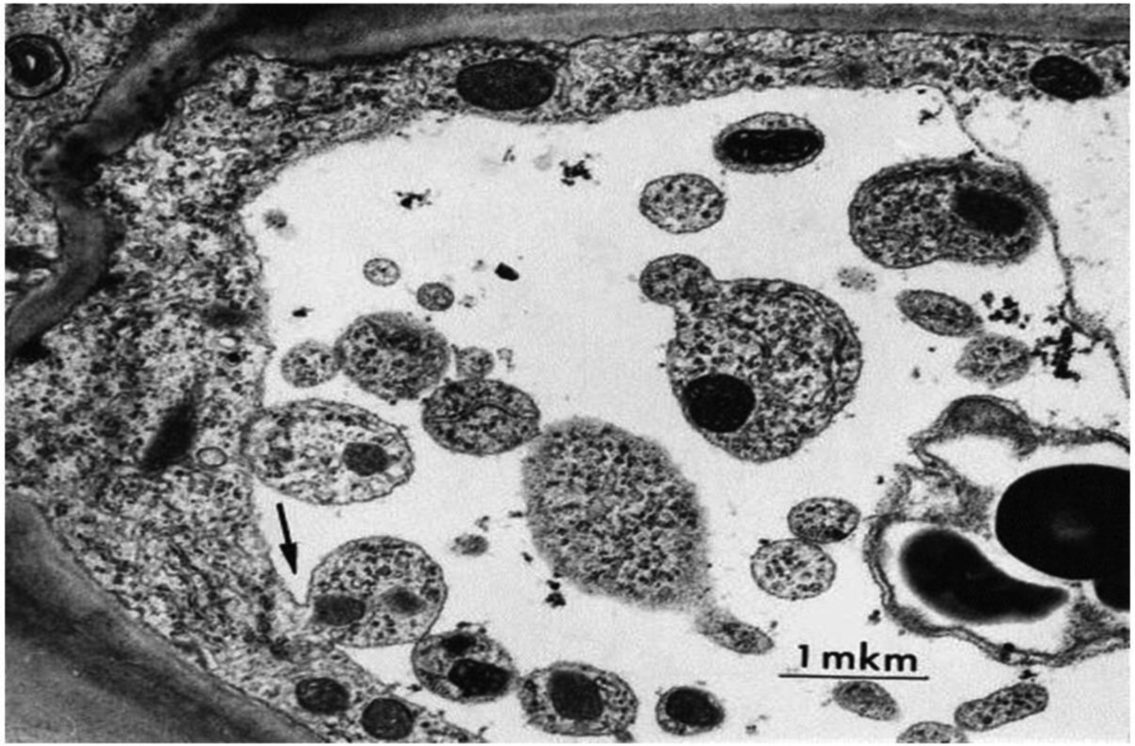
Bakeeva LE, Kirnos MD, Aleksandrushkina NI, et al. (1999) Subcellular reorganization of mitochondria producing heavy DNA in aging wheat coleoptiles. FEBS Lett 457: 122-125. doi: 10.1016/S0014-5793(99)01025-X
![]() |
[24] |
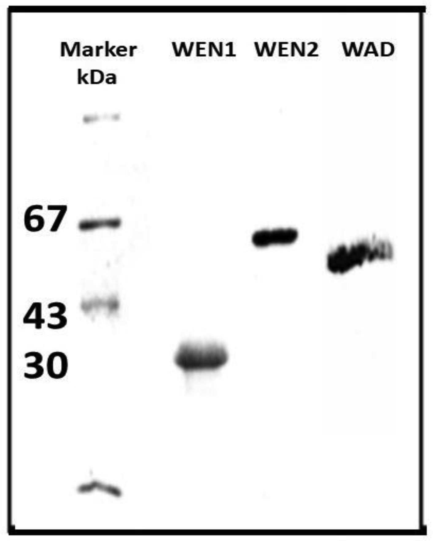
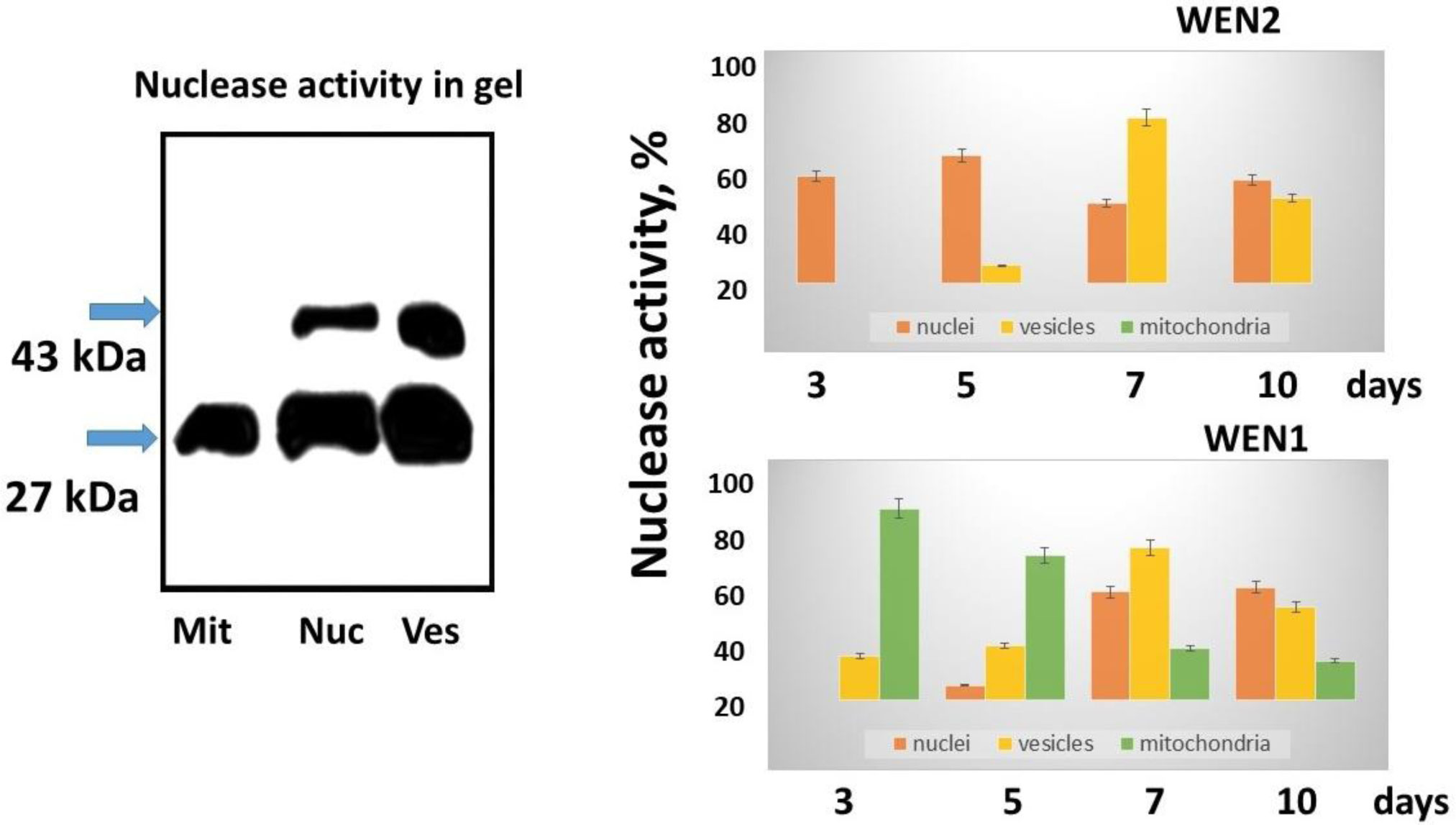
Fedoreyeva LI, Sobolev DE, Vanyushin BF (2007) Wheat endonuclease WEN1 depent on S-adenosyl-L-methionine and sensitive to DNA methylation status. Epigenetics 2: 50-53. doi: 10.4161/epi.2.1.3933
![]() |
[25] | Fedoreyeva LI, Sobolev DE, Vanyushin BF (2008) S-adenosyl-L-methionine dependent and sensitive to the status of DNA methylation endonuclease WEN2 from wheat coleoptiles. Biochemistry (Russian) 73: 1243-1251. |
[26] |
Fedoreyeva LI, Vanyushin B F (2002) N6-Adenine DNA-methyltransferase in wheat seedlings. FEBS Lett 514: 305-308. doi: 10.1016/S0014-5793(02)02384-0
![]() |
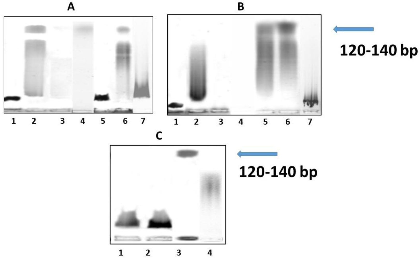
[27] | Kirnos MD, Aleksandrushkina NI, Vanyushin BF (1997) Apoptosis in cells of the first leaf and coleoptile of wheat seedlings: internucleosomal fragmentation of the genome and synthesis of heavy oligonucleosomal size of DNA fragments. Biochemistry (Russian) 62: 1008-1014. |
[28] |
Bradford MM (1976) A rapid and sensitive method for the quantitation of microgram quantities of protein utilizing the principle of protein-dye binding. Analyt Biochem 72: 248-254. doi: 10.1016/0003-2697(76)90527-3
![]() |
[29] |
Laemmli UK (1970) Cleavage of structural proteins during the assembly of the head of bacteriophage T4. Nature 227: 680-685. doi: 10.1038/227680a0
![]() |
[30] |
Bannister D, Glover SW (1968) Restriction and modification of bacteriophages by R strains of Escherichia coli K-12. Biochem Biophys Res Commun 30: 735-738. doi: 10.1016/0006-291X(68)90575-5
![]() |
[31] |
Vertino PM (1999) Eukaryotic DNA methyltransferases. S-Adenosylmethionine-dependent Methyltransferases: Structures and Functions 341-372. doi: 10.1142/9789812813077_0012
![]() |
[32] |
Bist P, Sistla S, Krishnamurthy V, et al. (2001) S-Adenosyl-L-methionine is required for DNA cleavage by type III restriction enzymes. J Mol Biol 310: 93-109. doi: 10.1006/jmbi.2001.4744
![]() |
[33] |
Cowan JA (2002) Structural and catalytic chemistry of magnesium-dependent enzymes. Biometals 15: 225-235. doi: 10.1023/A:1016022730880
![]() |
[34] | Lyons TJ, Eide DJ (2006) Transport and storage of metal ions in biology. Biological Inorganic Chemistry: Structure and Reactivity 57-77. |
[35] |
Maguire ME, Cowan JA (2002) Magnesium chemistry and biochemistry. Biometals 15: 203-210. doi: 10.1023/A:1016058229972
![]() |
[36] |
Romani A, Scarpa A (1992) Regulation of cell magnesium. Arch Biochem Biophys 298: 1-12. doi: 10.1016/0003-9861(92)90086-C
![]() |
[37] | Kirnos MD, Aleksandrushkina NI, Goremykin VV, et al. (1992) “Heavy” mitochondrial DNA in higher plants. Biochemistry (Russian) 57: 1566-1673. |
[38] | Aleksandrushkina NI, Kudryashova IB, Kirnos MD, et al. (1990) Synthesis and methylation at adenine residues of “heavy” miniplasmids of mitochondrial DNA in coleoptile and leaves of wheat seedlings. The influence of phytohormones. Biochemistry (Russian) 55: 2038-2045. |
[39] |
Kirnos MD, Alexandrushkina NI, Zagorskaya GYa, et al. (1992) Superproduction of heavy minicircular mitochondrial DNA in aging wheat coleoptiles. FEBS Lett 298: 109-112. doi: 10.1016/0014-5793(92)80033-D
![]() |
1. | Emadidin Gahalla Mohmed Elmahdi, Jianfei Huang, A linearized finite difference scheme for time–space fractional nonlinear diffusion-wave equations with initial singularity, 2022, 0, 1565-1339, 10.1515/ijnsns-2021-0388 | |
2. | Emadidin Gahalla Mohmed Elmahdi, Jianfei Huang, EFFICIENT NUMERICAL SOLUTION OF TWO-DIMENSIONAL TIME-SPACE FRACTIONAL NONLINEAR DIFFUSION-WAVE EQUATIONS WITH INITIAL SINGULARITY, 2022, 12, 2156-907X, 831, 10.11948/20210444 | |
3. | Chaeyoung Lee, Seokjun Ham, Youngjin Hwang, Soobin Kwak, Junseok Kim, An explicit fourth-order accurate compact method for the Allen-Cahn equation, 2024, 9, 2473-6988, 735, 10.3934/math.2024038 | |
4. | Emadidin Gahalla Mohmed Elmahdi, Yang Yi, Jianfei Huang, Two linearized difference schemes on graded meshes for the time-space fractional nonlinear diffusion-wave equation with an initial singularity, 2025, 100, 0031-8949, 015215, 10.1088/1402-4896/ad95c4 |
τ=h | α=1.25 | α=1.5 | α=1.75 | CPU time | |||
error | order | error | order | error | order | mean | |
1/5 | 6.6627×10⁻² | 7.8031×10⁻² | 8.9815×10⁻² | 0.0896 | |||
1/10 | 1.8412×10⁻² | 1.8555 | 2.1839×10⁻² | 1.8371 | 2.5456×10⁻² | 1.8190 | 0.0973 |
1/20 | 4.8132×10⁻³ | 1.9355 | 5.7273×10⁻³ | 1.9310 | 6.6917×10⁻³ | 1.9275 | 0.0994 |
1/40 | 1.2137×10⁻³ | 1.9876 | 1.4621×10⁻³ | 1.9698 | 1.7210×10⁻³ | 1.9591 | 0.1359 |
τ | α=1.25 | α=1.5 | α=1.75 | CPU time | |||
error | order | error | order | error | order | mean | |
1/5 | 7.0844×10⁻² | 8.2130×10⁻² | 9.3783×10⁻² | 0.5852 | |||
1/10 | 1.9012×10⁻² | 1.8977 | 2.2432×10⁻² | 1.8724 | 2.6040×10⁻² | 1.8486 | 1.0501 |
1/20 | 4.9405×10⁻³ | 1.9442 | 5.8537×10⁻³ | 1.9381 | 6.8169×10⁻³ | 1.9335 | 2.4071 |
1/40 | 1.2435×10⁻³ | 1.9903 | 1.4917×10⁻³ | 1.9724 | 1.7504×10⁻³ | 1.9615 | 6.7799 |
h | α=1.25 | α=1.5 | α=1.75 | CPU time | |||
error | order | error | order | error | order | mean | |
1/5 | 4.7813×10⁻³ | 4.7510×10⁻³ | 4.7111×10⁻³ | 2.2382 | |||
1/10 | 6.1943×10⁻⁴ | 2.9484 | 6.1518×10⁻⁴ | 2.9492 | 6.0963×10⁻⁴ | 2.9501 | 2.2952 |
1/20 | 1.2773×10⁻⁴ | 2.2778 | 1.2654×10⁻⁴ | 2.2815 | 1.2503×10⁻⁴ | 2.2857 | 2.5410 |
1/40 | 2.8950×10⁻⁵ | 2.1415 | 2.8363×10⁻⁵ | 2.1575 | 2.7665×10⁻⁵ | 2.1761 | 3.4293 |
τ | α=1.25 | α=1.5 | α=1.75 | CPU time | |||
error | order | error | order | error | order | mean | |
1/5 | 7.0844×10⁻² | 8.2129×10⁻² | 9.3783×10⁻² | 0.9501 | |||
1/10 | 1.9012×10⁻² | 1.8978 | 2.2432×10⁻² | 1.8724 | 2.6040×10⁻² | 1.8486 | 2.3622 |
1/20 | 4.9407×10⁻³ | 1.9441 | 5.8538×10⁻³ | 1.9381 | 6.8169×10⁻³ | 1.9335 | 7.6793 |
1/40 | 1.2436×10⁻³ | 1.9901 | 1.4919×10⁻³ | 1.9723 | 1.7506×10⁻³ | 1.9612 | 28.9326 |
h | α=1.25 | α=1.5 | α=1.75 | CPU time | |||
error | order | error | order | error | order | mean | |
1/5 | 3.8110×10⁻³ | 3.7871×10⁻³ | 3.7555×10⁻³ | 12.5566 | |||
1/10 | 2.5308×10⁻⁴ | 3.9125 | 2.5141×10⁻⁴ | 3.9130 | 2.4922×10⁻⁴ | 3.9135 | 14.0490 |
1/20 | 2.2087×10⁻⁵ | 3.5183 | 2.1851×10⁻⁵ | 3.5243 | 2.1557×10⁻⁵ | 3.5312 | 18.1726 |
1/40 | 1.8261×10⁻⁶ | 3.5964 | 1.7163×10⁻⁶ | 3.6703 | 1.5904×10⁻⁶ | 3.7607 | 43.9104 |