The Gelfand problem for the Infinity Laplacian

Fernando Charro; Byungjae Son; Peiyong Wang; Fernando Charro; Byungjae Son; Peiyong Wang

doi:10.3934/mine.2023022

Mathematics in Engineering

2023, Volume 5, Issue 2: 1-28. doi: 10.3934/mine.2023022

Previous Article Next Article

Research article Special Issues

The Gelfand problem for the Infinity Laplacian

1.
Department of Mathematics, Wayne State University, 656 W. Kirby St., Detroit, MI 48202, USA
2.
Department of Mathematics and Statistics, University of Maine, Orono, ME 04469, USA

Received: 10 December 2021 Revised: 21 February 2022 Accepted: 22 February 2022 Published: 11 April 2022

We study the asymptotic behavior as $p\to\infty$ of the Gelfand problem

$\begin{equation*} \left\{ \begin{aligned} -&\Delta_{p} u = \lambda\,e^{u}&& \text{in}\ \Omega\subset \mathbb{R}^n\\ &u = 0 && \text{on}\ \partial\Omega. \end{aligned} \right. \end{equation*}$

Under an appropriate rescaling on $u$ and $\lambda$ , we prove uniform convergence of solutions of the Gelfand problem to solutions of

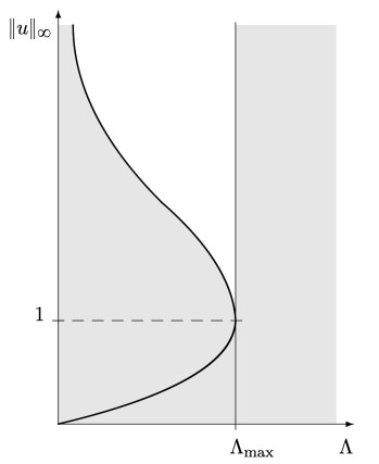
$\left\{ \begin{aligned} &\min\left\{|\nabla{}u|-\Lambda\,e^{u}, -\Delta_{\infty}u\right\} = 0&& \text{in}\ \Omega,\\ &u = 0\ &&\text{on}\ \partial\Omega. \end{aligned} \right.$

We discuss existence, non-existence, and multiplicity of solutions of the limit problem in terms of $\Lambda$ .

Keywords:

Citation: Fernando Charro, Byungjae Son, Peiyong Wang. The Gelfand problem for the Infinity Laplacian[J]. Mathematics in Engineering, 2023, 5(2): 1-28. doi: 10.3934/mine.2023022

Related Papers:

[1]	Chentong Li, Jinyan Wang, Jinhu Xu, Yao Rong . The Global dynamics of a SIR model considering competitions among multiple strains in patchy environments. Mathematical Biosciences and Engineering, 2022, 19(5): 4690-4702. doi: 10.3934/mbe.2022218
[2]	Xue-Zhi Li, Ji-Xuan Liu, Maia Martcheva . An age-structured two-strain epidemic model with super-infection. Mathematical Biosciences and Engineering, 2010, 7(1): 123-147. doi: 10.3934/mbe.2010.7.123
[3]	Matthew D. Johnston, Bruce Pell, David A. Rubel . A two-strain model of infectious disease spread with asymmetric temporary immunity periods and partial cross-immunity. Mathematical Biosciences and Engineering, 2023, 20(9): 16083-16113. doi: 10.3934/mbe.2023718
[4]	Ali Mai, Guowei Sun, Lin Wang . The impacts of dispersal on the competition outcome of multi-patch competition models. Mathematical Biosciences and Engineering, 2019, 16(4): 2697-2716. doi: 10.3934/mbe.2019134
[5]	Abdelrazig K. Tarboush, Jing Ge, Zhigui Lin . Coexistence of a cross-diffusive West Nile virus model in a heterogenous environment. Mathematical Biosciences and Engineering, 2018, 15(6): 1479-1494. doi: 10.3934/mbe.2018068
[6]	Azmy S. Ackleh, Mark L. Delcambre, Karyn L. Sutton, Don G. Ennis . A structured model for the spread of Mycobacterium marinum: Foundations for a numerical approximation scheme. Mathematical Biosciences and Engineering, 2014, 11(4): 679-721. doi: 10.3934/mbe.2014.11.679
[7]	Nancy Azer, P. van den Driessche . Competition and Dispersal Delays in Patchy Environments. Mathematical Biosciences and Engineering, 2006, 3(2): 283-296. doi: 10.3934/mbe.2006.3.283
[8]	Junjing Xiong, Xiong Li, Hao Wang . The survival analysis of a stochastic Lotka-Volterra competition model with a coexistence equilibrium. Mathematical Biosciences and Engineering, 2019, 16(4): 2717-2737. doi: 10.3934/mbe.2019135
[9]	Yanxia Dang, Zhipeng Qiu, Xuezhi Li . Competitive exclusion in an infection-age structured vector-host epidemic model. Mathematical Biosciences and Engineering, 2017, 14(4): 901-931. doi: 10.3934/mbe.2017048
[10]	Azmy S. Ackleh, Shuhua Hu . Comparison between stochastic and deterministic selection-mutation models. Mathematical Biosciences and Engineering, 2007, 4(2): 133-157. doi: 10.3934/mbe.2007.4.133

Abstract

We study the asymptotic behavior as $p\to\infty$ of the Gelfand problem

$\begin{equation*} \left\{ \begin{aligned} -&\Delta_{p} u = \lambda\,e^{u}&& \text{in}\ \Omega\subset \mathbb{R}^n\\ &u = 0 && \text{on}\ \partial\Omega. \end{aligned} \right. \end{equation*}$

Under an appropriate rescaling on $u$ and $\lambda$ , we prove uniform convergence of solutions of the Gelfand problem to solutions of

$\left\{ \begin{aligned} &\min\left\{|\nabla{}u|-\Lambda\,e^{u}, -\Delta_{\infty}u\right\} = 0&& \text{in}\ \Omega,\\ &u = 0\ &&\text{on}\ \partial\Omega. \end{aligned} \right.$

We discuss existence, non-existence, and multiplicity of solutions of the limit problem in terms of $\Lambda$ .

References

[1]	B. Abdellaoui, I. Peral, Existence and nonexistence results for quasilinear elliptic equations involving the $p$ -Laplacian with a critical potential, Ann. Mat. Pura Appl. IV. Ser., 182 (2003), 247–270. https://doi.org/10.1007/s10231-002-0064-y doi: 10.1007/s10231-002-0064-y
[2]	A. Anane, J. L. Lions, Simplicitè et isolation de la premiere valeur propre du $p$ -laplacien avec poids, C. R. Acad. Sci. Paris Sér. I Math., 305 (1987), 725–728.
[3]	T. Bhattacharya, E. DiBenedetto, J. Manfredi, Limit as $p\rightarrow \infty$ of $\Delta_{p}u_p = f$ and related extremal problems, Rend. Sem. Mat. Univ. Politec. Torino, 1989, 15–68.
[4]	M. Bocea, M. Mihǎilescu, Existence of nonnegative viscosity solutions for a class of problems involving the $\infty$ -Laplacian, Nonlinear Differ. Equ. Appl., 23 (2016), 11. https://doi.org/10.1007/s00030-016-0373-2 doi: 10.1007/s00030-016-0373-2
[5]	G. Bratu, Sur les équations intégrales non linéaires, Bulletin de la S. M. F., 42 (1914), 113–142.
[6]	H. Brezis, L. Oswald, Remarks on sublinear elliptic equations, Nonlinear Anal. Theor., 10 (1986), 55–64. https://doi.org/10.1016/0362-546X(86)90011-8 doi: 10.1016/0362-546X(86)90011-8
[7]	X. Cabré, M. Sanchón, Semi-stable and extremal solutions of reaction equations involving the $p$ -Laplacian, Commun. Pure Appl. Anal., 6 (2007), 43–67. https://doi.org/10.3934/cpaa.2007.6.43 doi: 10.3934/cpaa.2007.6.43
[8]	S. Chandrasekhar, An introduction to the study of stellar structures, New York: Dover, 1957.
[9]	S. Chanillo, M. Kiessling, Surfaces with prescribed Gauss curvature, Duke Math. J., 105 (2000), 309–353. https://doi.org/10.1215/S0012-7094-00-10525-X doi: 10.1215/S0012-7094-00-10525-X
[10]	F. Charro, E. Parini, Limits as $p\to\infty$ of $p$ -laplacian problems with a superdiffusive power-type nonlinearity: positive and sign-changing solutions, J. Math. Anal. Appl., 372 (2010), 629–644. https://doi.org/10.1016/j.jmaa.2010.07.005 doi: 10.1016/j.jmaa.2010.07.005
[11]	F. Charro, E. Parini, Limits as $p\to\infty$ of $p$ -laplacian eigenvalue problems perturbed with a concave or convex term, Calc. Var., 46 (2013), 403–425. https://doi.org/10.1007/s00526-011-0487-7 doi: 10.1007/s00526-011-0487-7
[12]	F. Charro, I. Peral, Limit branch of solutions as $p\rightarrow \infty$ for a family of sub-diffusive problems related to the p-laplacian, Commun. Part. Diff. Eq., 32 (2007), 1965–1981. https://doi.org/10.1080/03605300701454792 doi: 10.1080/03605300701454792
[13]	F. Charro, I. Peral, Limits as $p\to\infty$ of $p$ -Laplacian concave-convex problems, Nonlinear Anal. Theor., 75 (2012), 2637–2659. https://doi.org/10.1016/j.na.2011.11.009 doi: 10.1016/j.na.2011.11.009
[14]	M. G. Crandall, H. Ishii, P. L. Lions, User's guide to viscosity solutions of second order partial differential equations, Bull. Amer. Math. Soc., 27 (1992), 1–67. https://doi.org/10.1090/S0273-0979-1992-00266-5 doi: 10.1090/S0273-0979-1992-00266-5
[15]	J. Dávila, Singular solutions of semi-linear elliptic problems, In: Handbook of differential equations: stationary partial differential equations, Amsterdam: Elsevier/North-Holland, 2008, 83–176. https://doi.org/10.1016/S1874-5733(08)80019-8
[16]	M. Del Pino, J. Dolbeault, M. Musso, Multiple bubbling for the exponential nonlinearity in the slightly supercritical case, Commun. Pure Appl. Anal., 5 (2006), 463–482. https://doi.org/10.3934/cpaa.2006.5.463 doi: 10.3934/cpaa.2006.5.463
[17]	R. Emden, Gaskugeln: Anwendungen der mechanischen Wärmetheorie auf kosmologische und meteorologische Probleme (German), Germany: B. G. Teubner, 1907.
[18]	N. Fukagai, M. Ito, K. Narukawa, Limit as $p\rightarrow \infty$ of $p$ -Laplace eigenvalue problems and $L^\infty$ -inequality of the Poincare type, Differ. Integral Equ., 12 (1999), 183–206.
[19]	J. P. García Azorero, I. Peral, Existence and nonuniqueness for the p-laplacian: nonlinear eigenvalues, Commun. Part. Diff. Eq., 12 (1987), 1389–1430.
[20]	J. García Azorero, I. Peral Alonso, On a Emden-Fowler type equation, Nonlinear Anal. Theor., 18 (1992), 1085–1097. https://doi.org/10.1016/0362-546X(92)90197-M doi: 10.1016/0362-546X(92)90197-M
[21]	J. García Azorero, I. Peral Alonso, J. P. Puel, Quasilinear problems with exponential growth in the reaction term, Nonlinear Anal. Theor., 22 (1994), 481–498. https://doi.org/10.1016/0362-546X(94)90169-4 doi: 10.1016/0362-546X(94)90169-4
[22]	I. M. Gel'fand, Some problems in the theory of quasilinear equations, Amer. Math. Soc. Trans., 29 (1963), 295–381.
[23]	J.-F. Grosjean, $p$ -Laplace operator and diameter of manifolds, Ann. Glob. Anal. Geom., 28 (2005), 257–270. https://doi.org/10.1007/s10455-005-6637-4 doi: 10.1007/s10455-005-6637-4
[24]	J. Jacobsen, K. Schmitt, The Liouville-Bratu-Gelfand problem for radial operators, J. Differ. Equations, 184 (2002), 283–298. https://doi.org/10.1006/jdeq.2001.4151 doi: 10.1006/jdeq.2001.4151
[25]	R. Jensen, Uniqueness of Lipschitz extensions: Minimizing the sup norm of the gradient, Arch. Rational Mech. Anal., 123 (1993), 51–74. https://doi.org/10.1007/BF00386368 doi: 10.1007/BF00386368
[26]	D. D. Joseph, T. S. Lundgren, Quasilinear Dirichlet problems driven by positive sources, Arch. Rational Mech. Anal., 49 (1973), 241–269. https://doi.org/10.1007/BF00250508 doi: 10.1007/BF00250508
[27]	P. Juutinen, Minimization problems for Lipschitz functions via viscosity solutions, Helsinki: Suomalainen Tiedeakatemia, 1998.
[28]	P. Juutinen, Principal eigenvalue of a badly degenerate operator, J. Differ. Equations, 236 (2007), 532–550. https://doi.org/10.1016/j.jde.2007.01.020 doi: 10.1016/j.jde.2007.01.020
[29]	P. Juutinen, P. Lindqvist, On the higher eigenvalues for the $\infty$ -eigenvalue problem, Calc. Var., 23 (2005), 169–192. https://doi.org/10.1007/s00526-004-0295-4 doi: 10.1007/s00526-004-0295-4
[30]	P. Juutinen, P. Lindqvist, J. Manfredi, The $\infty$ -eigenvalue problem, Arch. Rational Mech. Anal., 148 (1999), 89–105. https://doi.org/10.1007/s002050050157 doi: 10.1007/s002050050157
[31]	B. Kawohl, On a family of torsional creep problems, J. Reine Angew. Math., 410 (1990), 1–22.
[32]	P. Lindqvist, On the equation $\text{div}\left(\|\nabla u\|^{p-2} \nabla u\right)+\lambda\|u\|^{p-2} u = 0$ , Proc. Amer. Math. Soc., 109 (1990), 157–164. https://doi.org/10.1090/S0002-9939-1990-1007505-7 doi: 10.1090/S0002-9939-1990-1007505-7
[33]	P. Lindqvist, Addendum: "On the equation $\text{div}\left(\|\nabla u\|^{p-2} \nabla u\right)+\lambda\|u\|^{p-2} u = 0$ '' [Proc. Amer. Math. Soc. 109 (1990), no. 1,157–164; MR1007505 (90h: 35088)], Proc. Amer. Math. Soc., 116 (1992), 583–584. https://doi.org/10.1090/S0002-9939-1992-1139483-6
[34]	P. Lindqvist, J. Manfredi, The Harnack inequality for $\infty$ -harmonic functions, Electron. J. Diff. Eqns., 5 (1995), 1–5.
[35]	P. Lindqvist, J. Manfredi, Note on $\infty$ -superharmonic functions, Revista Matemática de la Universidad Complutense de Madrid, 10 (1997), 471–480.
[36]	P. L. Lions, On the existence of positive solutions of semilinear elliptic equations, SIAM Rev., 24 (1982), 441–467. https://doi.org/10.1137/1024101 doi: 10.1137/1024101
[37]	J. Liouville, Sur l'équation aux différences partielles $\frac{d^2\log\lambda}dudv\pm \frac{\lambda}{2a^2} = 0$ , Journal de mathématiques pures et appliquées 1re série, 18 (1853), 71–72.
[38]	M. Mihǎilescu, D. Stancu-Dumitru, C. Varga, The convergence of nonnegative solutions for the family of problems $-\Delta_p u = \lambda e^u$ as $p\to\infty$ , ESAIM: COCV, 24 (2018), 569–578. https://doi.org/10.1051/cocv/2017048 doi: 10.1051/cocv/2017048
[39]	I. Peral, Some results on quasilinear elliptic equations: growth versus shape, In: Proceedings of the second school of nonlinear functional analysis and applications to differential equations, Trieste: World Scientific, 1998,153–202.
[40]	O. W. Richardson, The emission of electricity from hot Bodies, India: Longmans, Green and Company, 1921.
[41]	M. Sanchón, Regularity of the extremal solution of some nonlinear elliptic problems involving the $p$ -Laplacian, Potential Anal., 27 (2007), 217–224. https://doi.org/10.1007/s11118-007-9053-5 doi: 10.1007/s11118-007-9053-5
[42]	G. W. Walker, Some problems illustrating the forms of nebulae, Proc. R. Soc. Lond. A, 91 (1915), 410–420. https://doi.org/10.1098/rspa.1915.0032 doi: 10.1098/rspa.1915.0032
[43]	Y. Yu, Some properties of the ground states of the infinity Laplacian, Indiana Univ. Math. J., 56 (2007), 947–964.

This article has been cited by:

1.	Yixiang Wu, Necibe Tuncer, Maia Martcheva, Coexistence and competitive exclusion in an SIS model with standard incidence and diffusion, 2017, 22, 1553-524X, 1167, 10.3934/dcdsb.2017057
2.	Junping Shi, Yixiang Wu, Xingfu Zou, Coexistence of Competing Species for Intermediate Dispersal Rates in a Reaction–Diffusion Chemostat Model, 2020, 32, 1040-7294, 1085, 10.1007/s10884-019-09763-0
3.	Yixiang Wu, Xingfu Zou, Asymptotic profiles of steady states for a diffusive SIS epidemic model with mass action infection mechanism, 2016, 261, 00220396, 4424, 10.1016/j.jde.2016.06.028
4.	Lin Zhao, Zhi-Cheng Wang, Shigui Ruan, Dynamics of a time-periodic two-strain SIS epidemic model with diffusion and latent period, 2020, 51, 14681218, 102966, 10.1016/j.nonrwa.2019.102966
5.	Jing Ge, Ling Lin, Lai Zhang, A diffusive SIS epidemic model incorporating the media coverage impact in the heterogeneous environment, 2017, 22, 1553-524X, 2763, 10.3934/dcdsb.2017134
6.	Yuan Lou, Rachidi B. Salako, Control Strategies for a Multi-strain Epidemic Model, 2022, 84, 0092-8240, 10.1007/s11538-021-00957-6
7.	Jinsheng Guo, Shuang-Ming Wang, Threshold dynamics of a time-periodic two-strain SIRS epidemic model with distributed delay, 2022, 7, 2473-6988, 6331, 10.3934/math.2022352
8.	Rachidi B. Salako, Impact of population size and movement on the persistence of a two-strain infectious disease, 2023, 86, 0303-6812, 10.1007/s00285-022-01842-z
9.	Yuan Lou, Rachidi B. Salako, Mathematical analysis of the dynamics of some reaction-diffusion models for infectious diseases, 2023, 370, 00220396, 424, 10.1016/j.jde.2023.06.018
10.	Jonas T. Doumatè, Tahir B. Issa, Rachidi B. Salako, Competition-exclusion and coexistence in a two-strain SIS epidemic model in patchy environments, 2023, 0, 1531-3492, 0, 10.3934/dcdsb.2023213
11.	Azmy S. Ackleh, Nicolas Saintier, Aijun Zhang, A multiple-strain pathogen model with diffusion on the space of Radon measures, 2025, 140, 10075704, 108402, 10.1016/j.cnsns.2024.108402
12.	Jamal Adetola, Keoni G. Castellano, Rachidi B. Salako, Dynamics of classical solutions of a multi-strain diffusive epidemic model with mass-action transmission mechanism, 2025, 90, 0303-6812, 10.1007/s00285-024-02167-9

Reader Comments

Your name:*

Email:*
© 2023 the Author(s), licensee AIMS Press. This is an open access article distributed under the terms of the Creative Commons Attribution License (http://creativecommons.org/licenses/by/4.0)

通讯作者: 陈斌, bchen63@163.com

1.
沈阳化工大学材料科学与工程学院沈阳 110142

Mathematics in Engineering

1.3 2.9

Metrics

Article views(2463) PDF downloads(229) Cited by(0)

Preview PDF

Download XML

Export Citation

Article outline

Show full outline

Mathematics in Engineering

The Gelfand problem for the Infinity Laplacian

Related Papers:

Abstract

References

This article has been cited by:

Reader Comments

通讯作者: 陈斌, bchen63@163.com

Metrics

Figures and Tables

Other Articles By Authors

Catalog

Abstract

References

Mathematics in Engineering

The Gelfand problem for the Infinity Laplacian

Related Papers:

Abstract

References

This article has been cited by:

Reader Comments

通讯作者: 陈斌, bchen63@163.com

Metrics

Figures and Tables

Other Articles By Authors

Related pages

Tools

Export File

Citation

Format

Content

Catalog

Abstract

References