The high density of commercial aviation operations in Europe makes significant contributions to the emission of noise, greenhouse gases, and air pollutants. A key source of information which can be used in efforts to quantify these contributions is the OpenSky Network (OSN), which publishes automatic dependent surveillance - broadcast (ADS-B) data at time resolutions of up to one data point per second. This data can be used to reconstruct ground tracks and flight profiles, which can, in turn, be used to estimate local noise exposure, exhaust emissions, and local air quality. The use of such data in the reconstruction of departure flight paths is limited, however, by the lack of thrust settings and take-off weights. For this reason, a mixed analysis-synthesis approach was developed, in previous research, to reconstruct flight profiles by optimizing published departure procedures parameterized in terms of aircraft thrust settings and take-off weight, and departure procedure parameters. The approach can be used to reconstruct large numbers of flight profiles, throughout significant time windows, from open-source ADS-B data. Errors in the estimations of the parameters can lead to errors in the flight profile calculation which will propagate through to follow-on noise, fuel flow, and emissions calculations. In this paper, a global variance-based sensitivity analysis is presented, which evaluated the sensitivity of departure flight profile altitude to mixed analysis-synthesis flight profile parameters. The purpose was to improve understanding of the dominant sources of error and uncertainty in the flight profile reconstruction, and the influence of aspects of departure flight operations on resulting flight profiles. Analyses were presented for three different airports, Amsterdam Schiphol (EHAM), Dublin (EIDW) and Stockholm (ESSA) airports, considering departures of aircraft corresponding to the 737–800 and A320-211 aircraft classes.
Citation: James H. Page, Lorenzo Dorbolò, Marco Pretto, Alessandro Zanon, Pietro Giannattasio, Michele De Gennaro. Sensitivity analysis of mixed analysis-synthesis flight profile reconstruction[J]. Metascience in Aerospace, 2024, 1(4): 401-415. doi: 10.3934/mina.2024019
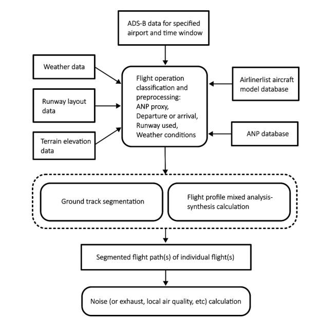
The high density of commercial aviation operations in Europe makes significant contributions to the emission of noise, greenhouse gases, and air pollutants. A key source of information which can be used in efforts to quantify these contributions is the OpenSky Network (OSN), which publishes automatic dependent surveillance - broadcast (ADS-B) data at time resolutions of up to one data point per second. This data can be used to reconstruct ground tracks and flight profiles, which can, in turn, be used to estimate local noise exposure, exhaust emissions, and local air quality. The use of such data in the reconstruction of departure flight paths is limited, however, by the lack of thrust settings and take-off weights. For this reason, a mixed analysis-synthesis approach was developed, in previous research, to reconstruct flight profiles by optimizing published departure procedures parameterized in terms of aircraft thrust settings and take-off weight, and departure procedure parameters. The approach can be used to reconstruct large numbers of flight profiles, throughout significant time windows, from open-source ADS-B data. Errors in the estimations of the parameters can lead to errors in the flight profile calculation which will propagate through to follow-on noise, fuel flow, and emissions calculations. In this paper, a global variance-based sensitivity analysis is presented, which evaluated the sensitivity of departure flight profile altitude to mixed analysis-synthesis flight profile parameters. The purpose was to improve understanding of the dominant sources of error and uncertainty in the flight profile reconstruction, and the influence of aspects of departure flight operations on resulting flight profiles. Analyses were presented for three different airports, Amsterdam Schiphol (EHAM), Dublin (EIDW) and Stockholm (ESSA) airports, considering departures of aircraft corresponding to the 737–800 and A320-211 aircraft classes.

| [1] | EUROCONTROL (2023) EUROCONTROL seven year forecast 2023-2029. Available from: https://www.eurocontrol.int/sites/default/files/2023-10/eurocontrol-seven-year-forecast-2023-2029-region-definition.pdf. |
| [2] | ICAO (2023) Global trends in aircraft noise. |
| [3] | European Commission (2024) Reducing emissions from aviation. Available: https://climate.ec.europa.eu/eu-action/transport/reducing-emissions-aviation_en. |
| [4] | ECAC.CEAC (2025) Report on Standard Method of Computing Noise Contours around Civil Airports Volume 1: Applications Guide. |
| [5] | ECAC.CEAC (2016) Report on Standard Method of Computing Noise Contours around Civil Airports Volume 2: Technical Guide. |
| [6] |
Pretto M, Giannattasio P, De Gennaro M (2022) Mixed analysis-synthesis approach for estimating airport noise from civil air traffic. Transport Res D-Tr E 106: 103248. https://doi.org/10.1016/j.trd.2022.103248 doi: 10.1016/j.trd.2022.103248

|
| [7] |
Pretto M, Dorbolò L, Giannattasio P, et al. (2024) Aircraft trajectory reconstruction and airport noise prediction from high-resolution flight tracking data. Transport Res D-Tr E 135: 104397. https://doi.org/10.1016/j.trd.2024.104397 doi: 10.1016/j.trd.2024.104397
|
| [8] | EUROCONTROL (2023) The aircraft noise and performance database (ANP) database: an international data resource for aircraft noise modellers. |
| [9] | EUROCONTROL (2024) IMPACT: integrated aircraft noise and emissions modelling platform. |
| [10] | Federal Aviation Administration (FAA) Aviation Environmental Design Tool (AEDT). Available from: https://aedt.faa.gov/. |
| [11] | Ollerhead JB (1992) The CAA Aircraft Noise Contour Model: ANCON Version 1, Cheltenham, UK: Civil Aviation Authority. |
| [12] | Rekkas C, Rees M (2008) Towards ADS-B implementation in Europe. in 2008 Tyrrhenian International Workshop on Digital Communications - Enhanced Surveillance of Aircraft and Vehicles, Capri, Italy. https://doi.org/10.1109/TIWDC.2008.4649019 |
| [13] | De Gennaro M, Zanon A, Kuehnelt H, et al. (2018) Big data for low-carbon transport: an overview of applications for designing the future of road and aerial transport, in 7th Transport Research Arena, Vienna. |
| [14] | Gagliardi P, Fredianelli L, Simonetti D, et al. (2017) ADS-B System as a Useful Tool for Testing and Redrawing Noise Management Strategies at Pisa Airport. Acta Acust United Acust 103: 543–551. |
| [15] | Flightradar24. Available from: https://www.flightradar24. |
| [16] | FlightAware. Available from: https://www.flightaware.com. |
| [17] | Plane Finder. Available from: https://planefinder.net/. |
| [18] | Airfleets.net. Available from: https://www.airfleets.net. |
| [19] |
Pretto M, Giannattasio P, De Gennaro M, et al. (2019) Web data for computing real-world noise from civil aviation. Transport Res D-Tr E 69: 224–249. https://doi.org/10.1016/j.trd.2019.01.022 doi: 10.1016/j.trd.2019.01.022
|
| [20] |
Pretto M, Giannattasio P, De Gennaro M, et al (2020) Forecasts of future scenarios for airport noise based on collection and processing of web data. Eur Transp Res Rev 12: 4. https://doi.org/10.1186/s12544-019-0389-x doi: 10.1186/s12544-019-0389-x
|
| [21] | Olive X (2019) Traffic: air traffic data processing with Python. |
| [22] |
Olive X (2019) Traffic, a toolbox for processing and analysing air traffic data. J Open Source Softw 4: 1518, 1–3. https://doi.org/10.21105/joss.01518 doi: 10.21105/joss.01518
|
| [23] |
Sun J, Ellerbroek J, Hoekstra JM (2019) WRAP: An open-source kinematic aircraft performance model. Transport Res C-Emer 98: 118–138. https://doi.org/10.1016/j.trc.2018.11.009 doi: 10.1016/j.trc.2018.11.009
|
| [24] | Schä fer M, Strohmeier M, Lenders V, et al. (2014) Bringing up OpenSky: A large-scale ADS-B sensor network for research, in IPSN-14 Proceedings of the 13th International Symposium on Information Processing in Sensor Networks, Berlin, Germany, 83–94. https://doi.org/10.1109/IPSN.2014.6846743 |
| [25] |
Pretto M, Dorbolò L, Giannattasio P (2023) (Poster) Exploiting high-resolution ADS-B data for flight operation reconstruction towards environmental impact assessment. J Open Aviat Sci 1. https://doi.org/10.59490/joas.2023.7208 doi: 10.59490/joas.2023.7208
|
| [26] | Airlinerlist. Available from: https://www.planelist.net/. |
| [27] | EASA – ANP (2023) Aircraft Noise and Performance (ANP) Data. |
| [28] |
Sobol IM (2001) Global sensitivity indices for nonlinear mathematical models and their Monte Carlo estimates. Math Comput Simulat 55: 271–280. https://doi.org/10.1016/S0378-4754(00)00270-6 doi: 10.1016/S0378-4754(00)00270-6
|
| [29] |
Saltelli A (2002) Making best use of model evaluations to compute sensitivity indices. Comput Phys Commun 145: 280–297. https://doi.org/10.1016/S0010-4655(02)00280-1 doi: 10.1016/S0010-4655(02)00280-1
|
| [30] | Campolongo F, Saltelli A, Cariboni J (2011) From screening to quantitative sensitivity analysis. A unified approach. Comput Phys Commun 182: 978–988. |
| [31] | OurAirports. Available from: https://ourairports.com/. |
| [32] | OpenStreetMap. Available from: https://www.openstreetmap.org. |


Figures(9) / Tables(3)
James H. Page, Lorenzo Dorbolò, Marco Pretto, Alessandro Zanon, Pietro Giannattasio, Michele De Gennaro. Sensitivity analysis of mixed analysis-synthesis flight profile reconstruction[J]. Metascience in Aerospace, 2024, 1(4): 401-415. doi: 10.3934/mina.2024019


 DownLoad: