Perspective on utilization of <i>Bacillus</i> species as plant probiotics for different crops in adverse conditions

Shubhra Singh; Douglas J. H. Shyu; Shubhra Singh; Douglas J. H. Shyu

doi:10.3934/microbiol.2024011

AIMS Microbiology

2024, Volume 10, Issue 1: 220-238. doi: 10.3934/microbiol.2024011

Previous Article Next Article

Review

Perspective on utilization of Bacillus species as plant probiotics for different crops in adverse conditions

Shubhra Singh ¹,
Douglas J. H. Shyu ^{2
,
,}

1.
Department of Tropical Agriculture and International Cooperation, National Pingtung University of Science and Technology, Pingtung 912301, Taiwan
2.
Department of Biological Science and Technology, National Pingtung University of Science and Technology, Pingtung 912301, Taiwan

Received: 23 November 2023 Revised: 21 February 2024 Accepted: 22 February 2024 Published: 13 March 2024

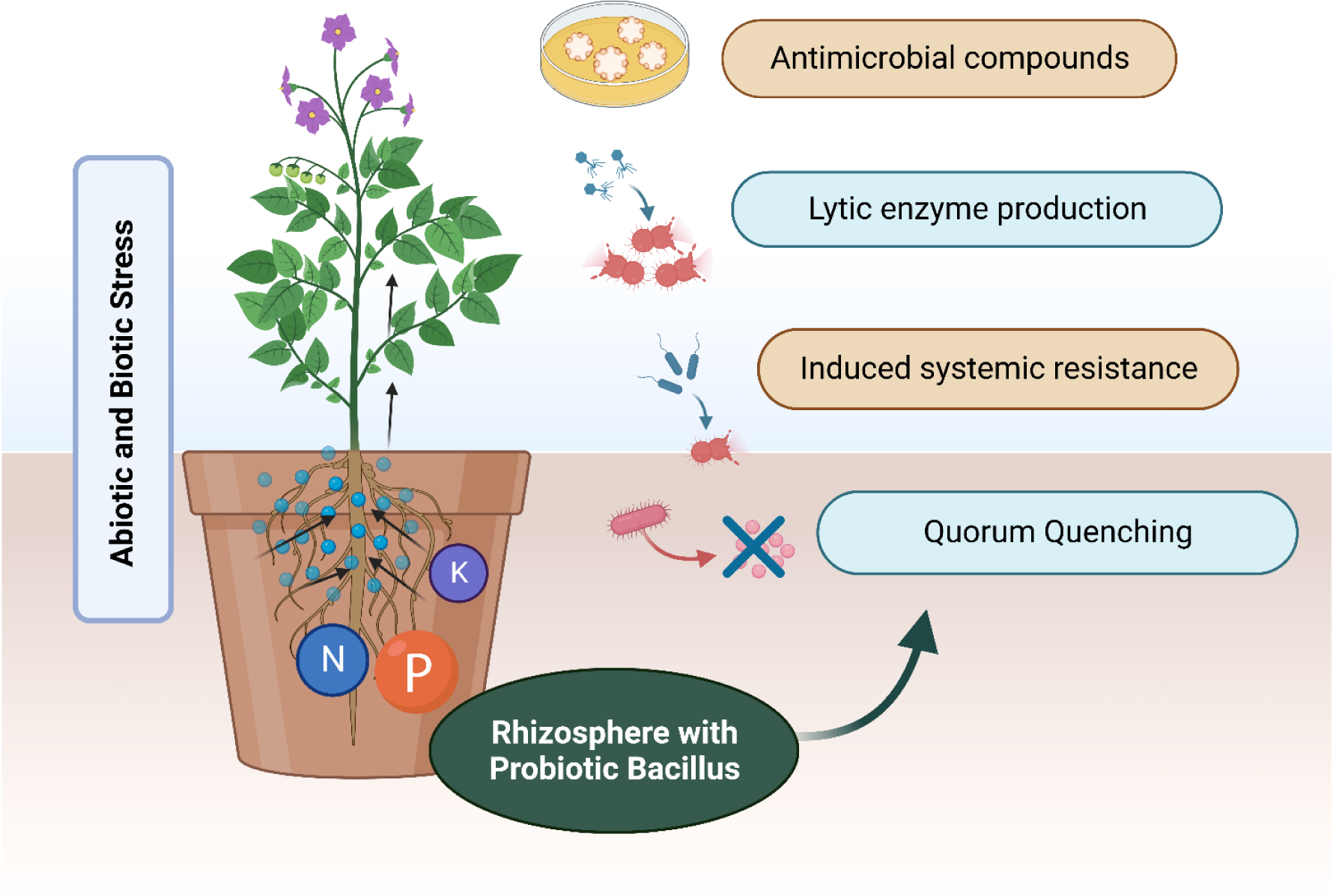
Plant probiotic bacteria are a versatile group of bacteria isolated from different environmental sources to improve plant productivity and immunity. The potential of plant probiotic-based formulations is successfully seen as growth enhancement in economically important plants. For instance, endophytic Bacillus species acted as plant growth-promoting bacteria, influenced crops such as cowpea and lady's finger, and increased phytochemicals in crops such as high antioxidant content in tomato fruits. The present review aims to summarize the studies of Bacillus species retaining probiotic properties and compare them with the conventional fertilizers on the market. Plant probiotics aim to take over the world since it is the time to rejuvenate and restore the soil and achieve sustainable development goals for the future. Comprehensive coverage of all the Bacillus species used to maintain plant health, promote plant growth, and fight against pathogens is crucial for establishing sustainable agriculture to face global change. Additionally, it will give the latest insight into this multifunctional agent with a detailed biocontrol mechanism and explore the antagonistic effects of Bacillus species in different crops.
- Bacillus species,
- crops,
- endophytes,
- plant growth-promoting bacteria,
- plant probiotics,
- sustainable agriculture
Citation: Shubhra Singh, Douglas J. H. Shyu. Perspective on utilization of Bacillus species as plant probiotics for different crops in adverse conditions[J]. AIMS Microbiology, 2024, 10(1): 220-238. doi: 10.3934/microbiol.2024011

Related Papers:

Abstract

Plant probiotic bacteria are a versatile group of bacteria isolated from different environmental sources to improve plant productivity and immunity. The potential of plant probiotic-based formulations is successfully seen as growth enhancement in economically important plants. For instance, endophytic Bacillus species acted as plant growth-promoting bacteria, influenced crops such as cowpea and lady's finger, and increased phytochemicals in crops such as high antioxidant content in tomato fruits. The present review aims to summarize the studies of Bacillus species retaining probiotic properties and compare them with the conventional fertilizers on the market. Plant probiotics aim to take over the world since it is the time to rejuvenate and restore the soil and achieve sustainable development goals for the future. Comprehensive coverage of all the Bacillus species used to maintain plant health, promote plant growth, and fight against pathogens is crucial for establishing sustainable agriculture to face global change. Additionally, it will give the latest insight into this multifunctional agent with a detailed biocontrol mechanism and explore the antagonistic effects of Bacillus species in different crops.

Acknowledgments

We would like to thank Mr. Liyu Chiang for his assistance.

Conflict of interest

The authors declare no conflict of interest.

Author Contributions

S.S.: Conceptualization, Investigation, Data Curation, Validation, Writing – Original Draft Preparation. D.J.H.S: Conceptualization, Supervision, Project Administration, Suggestion, and Writing – Review and Editing.

References

[1]	Hamilton-Miller JMT, Gibson GR, Bruck W (2003) Some insights into the derivation and early uses of the word ‘probiotic’. Br J Nutr 90: 845-845. https://doi.org/10.1079/BJN2003954
[2]	Jiménez-Gómez A, Celador-Lera L, Fradejas-Bayón M, et al. (2017) Plant probiotic bacteria enhance the quality of fruit and horticultural crops. AIMS Microbiol 3: 483-501. https://doi.org/10.3934/microbiol.2017.3.483
[3]	Carro L, Nouioui I (2017) Taxonomy and systematics of plant probiotic bacteria in the genomic era. AIMS Microbiol 3: 383-412. https://doi.org/10.3934/microbiol.2017.3.383
[4]	Yobo KS Utilisation of Bacillus spp. as Plant Probiotics (Doctoral dissertation) (2000). Available from: https://researchspace.ukzn.ac.za/server/api/core/bitstreams/bc94cab8-4472-4cac-84cd-2129b55d3108/content
[5]	Jimtha JC, Jishma P, Arathy GB, et al. (2016) Identification of plant growth promoting rhizosphere Bacillus sp. WG4 antagonistic to Pythium myriotylum and its enhanced antifungal effect in association with Trichoderma. J Soil Sci Plant Nutr 16: 578-590. https://doi.org/10.4067/S0718-95162016005000026
[6]	Miljaković D, Marinković J, Balešević-Tubić S (2020) The significance of Bacillus spp. In disease suppression and growth promotion of field and vegetable crops. Microorganisms 8: 1037. https://doi.org/10.3390/microorganisms8071037
[7]	Hashem A, Tabassum B, Fathi Abd_Allah E (2019) Bacillus subtilis: A plant-growth promoting rhizobacterium that also impacts biotic stress. Saudi J Biol Sci 26: 1291-1297. https://doi.org/10.1016/j.sjbs.2019.05.004
[8]	Song J, Kong ZQ, Zhang DD, et al. (2021) Rhizosphere microbiomes of potato cultivated under Bacillus subtilis treatment influence the quality of potato tubers. Int J Mol Sci 22: 12065. https://doi.org/10.3390/ijms222112065
[9]	Feng Y, Zhang Y, Shah OU, et al. (2023) Isolation and identification of endophytic bacteria Bacillus sp. ME9 that exhibits biocontrol activity against Xanthomonas phaseoli pv. manihotis. Biology (Basel) 9: 1231. https://doi.org/10.3390/biology12091231
[10]	Anckaert A, Arias AA, Hoff G (2021) The use of Bacillus spp. as bacterial biocontrol agents to control plant diseases. Burleigh Dodds Series In Agricultural Science. Cambridge: Burleigh Dodds Science Publishing. https://doi.org/10.19103/AS.2021.0093.10
[11]	Beauregard PB, Chai Y, Vlamakis H, et al. (2013) Bacillus subtilis biofilm induction by plant polysaccharides. Proc Natl Acad Sci U S A 110: 1621-1630. https://doi.org/10.1073/pnas.1218984110
[12]	Arnaouteli S, Bamford NC, Stanley-Wall NR, et al. (2021) Bacillus subtilis biofilm formation and social interactions. Nat Rev Microbiol 19: 600-614. https://doi.org/10.1038/s41579-021-00540-9
[13]	Liu H, Prajapati V, Prajapati S, et al. (2021) Comparative genome analysis of Bacillus amyloliquefaciens focusing on phylogenomics, functional traits, and prevalence of antimicrobial and virulence genes. Front Genet 12: 724217. https://doi.org/10.3389/fgene.2021.724217
[14]	Huang Q, Zhang Z, Liu Q, et al. (2021) SpoVG is an important regulator of sporulation and affects biofilm formation by regulating Spo0A transcription in Bacillus cereus 0–9. BMC Microbiol 21: 172. https://doi.org/10.1186/s12866-021-02239-6
[15]	García-Fraile P, Menéndez E, Rivas R (2015) Role of bacterial biofertilizers in agriculture and forestry. AIMS Bioeng 2: 183-205. https://doi.org/10.3934/bioeng.2015.3.183
[16]	Lopes MJ dos S, Dias-Filho MB, Gurgel ESC (2021) Successful plant growth-promoting microbes: Inoculation methods and abiotic factors. Front Sustain Food Syst 5: 656454. https://doi.org/10.3389/fsufs.2021.606454
[17]	Gahir S, Bharath P, Raghavendra AS (2021) Stomatal closure sets in motion long-term strategies of plant defense against microbial pathogens. Front Plant Sci 12: 761952. https://doi.org/10.3389/fpls.2021.761952
[18]	Herpell JB, Alickovic A, Diallo B, et al. (2023) Phyllosphere symbiont promotes plant growth through ACC deaminase production. ISME J 17: 1267-1277. https://doi.org/10.1038/s41396-023-01428-7
[19]	Orozco-Mosqueda M del C, Glick BR, Santoyo G (2020) ACC deaminase in plant growth-promoting bacteria (PGPB): An efficient mechanism to counter salt stress in crops. Microbiol Res 235: 126-439. https://doi.org/10.1016/j.micres.2020.126439
[20]	Jiang CH, Xie YS, Zhu K, et al. (2019) Volatile organic compounds emitted by Bacillus sp. JC03 promote plant growth through the action of auxin and strigolactone. Plant Growth Regul 87: 317-328. https://doi.org/10.1007/s10725-018-00473-z
[21]	Hassan AHA, Hozzein WN, Mousa ASM, et al. (2020) Heat stress as an innovative approach to enhance the antioxidant production in Pseudooceanicola and Bacillus isolates. Sci Rep 10: 15076. https://doi.org/10.1038/s41598-020-72054-y
[22]	Etesami H (2020) Plant-microbe interactions in plants and stress tolerance. Plant Life Under Changing Environment: Responses and Management. New York: Academic Press 355-396. https://doi.org/10.1016/B978-0-12-818204-8.00018-7
[23]	Maheshwari DK (2012) Bacteria in Agrobiology: Plant Probiotics. Switzerland: Springer Science & Business Media 325-363. https://doi.org/10.1007/978-3-642-27515-9
[24]	Lavelle P, Spain AV (2002) Soil Ecology. Dordrecht, Netherlands: Springer Nature BV. https://doi.org/10.1007/0-306-48162-6
[25]	Akhtar MS (2019) Salt Stress, Microbes, and Plant Interactions : Causes and Solution. Singapore: Springer Nature Singapore Pte Ltd.. https://doi.org/10.1007/978-981-13-8801-9
[26]	Yi J, Sheng G, Suo Z, et al. (2020) Biofertilizers with beneficial rhizobacteria improved plant growth and yield in chili (Capsicum annuum L.). World J Microbiol Biotechnol 36: 86. https://doi.org/10.1007/s11274-020-02863-w
[27]	Varma A, Tripathi S, Prasad R (2020) Plant Microbe Symbiosis. Cham, Switzerland: Springer. https://doi.org/10.1007/978-3-030-36248-5_1
[28]	Kutschera U, Khanna R (2016) Plant gnotobiology : Epiphytic microbes and sustainable agriculture. Plant SignalBehav 12: 1256529. https://doi.org/10.1080/15592324.2016.1256529
[29]	Bidondo LF, Bompadre J, Pergola M, et al. (2012) Differential interaction between two Glomus intraradices strains and a phosphate solubilizing bacterium in maize rhizosphere. Pedobiologia-Int J Soil Biol 55: 227-232. https://doi.org/10.1016/j.pedobi.2012.04.001
[30]	Kuan KB, Othman R, Rahim KA (2016) Plant growth-promoting rhizobacteria inoculation to enhance vegetative growth, nitrogen fixation and nitrogen remobilisation of maize under greenhouse conditions. PLoS ONE 11: e0152478. https://doi.org/10.1371/journal.pone.0152478
[31]	Chaves-Gómez JL, Chávez-Arias CC, Prado AMC, et al. (2021) Mixtures of biological control agents and organic additives improve physiological behavior in cape gooseberry plants under vascular wilt disease. Plants 10: 20-59. https://doi.org/10.3390/plants10102059
[32]	Kang SM, Radhakrishnan R, Lee KE, et al. (2015) Mechanism of plant growth promotion elicited by Bacillus sp. LKE15 in oriental melon. Acta Agric Scand Sect B Soil Plant Sci 65: 637-647. https://doi.org/10.1080/09064710.2015.1040830
[33]	Dursun A, Ekinci M, Dönmez MF (2010) Effects of foliar application of plant growth promoting bacterium on chemical contents, yield and growth of tomato (Lycopersicon esculentum L.) and cucumber (Cucumis sativus L.). Pakistan J Bot 42: 3349-3356. https://www.pakbs.org/pjbot/PDFs/42(5)/PJB42(5)3349.pdf
[34]	Barnawal D, Maji D, Bharti N, et al. (2013) ACC deaminase-containing Bacillus subtilis reduces stress ethylene-induced damage and improves mycorrhizal colonization and rhizobial nodulation in Trigonella foenum-graecum under drought stress. J Plant Growth Regul 32: 809-822. https://doi.org/10.1007/s00344-013-9347-3
[35]	Ashraf M, Hasnain S, Berge O, et al. (2004) Inoculating wheat seedlings with exopolysaccharide-producing bacteria restricts sodium uptake and stimulates plant growth under salt stress. Biol Fertil Soils 40: 157-162. https://doi.org/10.1007/s00374-004-0766-y
[36]	Kang SM, Radhakrishnan R, You YH, et al. (2014) Phosphate solubilizing Bacillus megaterium mj1212 regulates endogenous plant carbohydrates and amino acids contents to promote mustard plant growth. Indian J Microbiol 54: 427-433. https://doi.org/10.1007/s12088-014-0476-6
[37]	Radhakrishnan R, Lee IJ (2016) Gibberellins producing Bacillus methylotrophicus KE2 supports plant growth and enhances nutritional metabolites and food values of lettuce. Plant Physiol Biochem 109: 181-189. https://doi.org/10.1016/j.plaphy.2016.09.018
[38]	Pourbabaee AA, Bahmani E, Alikhani HA, et al. (2016) Promotion of wheat growth under salt stress by halotolerant bacteria containing ACC deaminase. J Agric Sci Technol 18: 855-864. https://jast.modares.ac.ir/article-23-11250-en.pdf
[39]	Xu M, Sheng J, Chen L, et al. (2014) Bacterial community compositions of tomato (Lycopersicum esculentum Mill.) seeds and plant growth promoting activity of ACC deaminase producing Bacillus subtilis (HYT-12-1) on tomato seedlings. World J Microbiol Biotechnol 30: 835-845. https://doi.org/10.1007/s11274-013-1486-y
[40]	Basheer J, Ravi A, Mathew J, et al. (2019) Assessment of plant-probiotic performance of novel endophytic Bacillus sp. in talc-based formulation. Probiotics Antimicrob Proteins 11: 256-263. https://doi.org/10.1007/s12602-018-9386-y
[41]	John C J, GE M, Noushad N (2021) Probiotic rhizospheric Bacillus sp. from Zingiber officinale Rosc. displays antifungal activity against soft rot pathogen Pythium sp. Curr Plant Biol 27: 100217. https://doi.org/10.1016/j.cpb.2021.100217
[42]	Chandrasekaran M, Chun SC, Oh JW, et al. (2019) Bacillus subtilis CBR05 for tomato (Solanum lycopersicum) fruits in South Korea as a novel plant probiotic bacterium (PPB): Implications from total phenolics, flavonoids, and carotenoids content for fruit quality. Agronomy 9: 838. https://doi.org/10.3390/agronomy9120838
[43]	Wu X, Li H, Wang Y, et al. (2020) Effects of bio-organic fertiliser fortiﬁed by Bacillus cereus QJ-1 on tobacco bacterial wilt control and soil quality improvement. Biocontrol Sci Technol 30: 351-369. https://doi.org/10.1080/09583157.2020.1711870
[44]	Subramani T, Krishnan S, Kaari M, et al. (2017) Efficacy of Bacillus-fortified organic fertilizer for controlling bacterial wilt (Ralstonia solanacearum) of tomato under protected cultivation in the tropical Islands. Ecol Environ Conserv 23: 968-972.
[45]	Zhou L, Song C, Muñoz CY, et al. (2021) Bacillus cabrialesii BH5 protects tomato plants against Botrytis cinerea by production of specific antifungal compounds. Front Microbiol 12: 707609. https://doi.org/10.3389/fmicb.2021.707609
[46]	Riera N, Handique U, Zhang Y, et al. (2017) Characterization of antimicrobial-producing beneficial bacteria isolated from Huanglongbing escape citrus trees. Front Microbiol 8: 2415. https://doi.org/10.3389/fmicb.2017.02415
[47]	Lu M, Chen Y, Li L, et al. (2022) Analysis and evaluation of the flagellin activity of Bacillus amyloliquefaciens Ba168 antimicrobial proteins against Penicillium expansum. Molecules 27: 4259. https://doi.org/10.3390/molecules27134259
[48]	Lin C, Tsai CH, Chen PY, et al. (2018) Biological control of potato common scab by Bacillus amyloliquefaciens Ba01. PLoS One 13: e0196520. https://doi.org/10.1371/journal.pone.0196520
[49]	Wu L, Wu H, Chen L, et al. (2015) Difficidin and bacilysin from Bacillus amyloliquefaciens FZB42 have antibacterial activity against Xanthomonas oryzae rice pathogens. Sci Rep 5: 12975. https://doi.org/10.1038/srep12975
[50]	Azaiez S, Ben Slimene I, Karkouch I, et al. (2018) Biological control of the soft rot bacterium Pectobacterium carotovorum by Bacillus amyloliquefaciens strain Ar10 producing glycolipid-like compounds. Microbiol Res 217: 23-33. https://doi.org/10.1016/j.micres.2018.08.013
[51]	Ben S, Kilani-feki O, Dammak M, et al. (2015) Efficacy of Bacillus subtilis V26 as a biological control agent against Rhizoctonia solani on potato. Comptes Rendus Biol 338: 784-792. https://doi.org/10.1016/j.crvi.2015.09.005
[52]	Parmar A, Sharma S (2018) Engineering design and mechanistic mathematical models: Standpoint on cutting edge drug delivery. Trends Anal Chem 100: 15-35. https://doi.org/10.1016/j.trac.2017.12.008
[53]	Uroz S, Dessaux Y, Oger P (2009) Quorum sensing and quorum quenching: The Yin and Yang of bacterial communication. ChemBioChem 10: 205-216. https://doi.org/10.1002/cbic.200800521
[54]	Khoiri S, Damayanti TA, Giyanto G (2017) Identification of quorum quenching bacteria and its biocontrol potential against soft rot disease bacteria, Dickeya dadantii. Agrivita 39: 45-55. http://doi.org/10.17503/agrivita.v39i1.633
[55]	Chong TM, Koh CL, Sam CK, et al. (2012) Characterization of quorum sensing and quorum quenching soil bacteria isolated from Malaysian tropical montane forest. Sensors 12: 4846-4859. https://doi.org/10.3390/s120404846
[56]	Van Oosten MJ, Pepe O, De Pascale S, et al. (2017) The role of biostimulants and bioeffectors as alleviators of abiotic stress in crop plants. Chem Biol Technol Agric 4: 1-12. https://doi.org/10.1186/s40538-017-0089-5
[57]	Chen W, Wu Z, Liu C, et al. (2023) Biochar combined with Bacillus subtilis SL-44 as an eco-friendly strategy to improve soil fertility, reduce Fusarium wilt, and promote radish growth. Ecotoxicol Environ Saf 251: 114-509. https://doi.org/10.1016/j.ecoenv.2023.114509
[58]	Chen W, Wu Z, He Y (2023) Isolation, purification, and identification of antifungal protein produced by Bacillus subtilis SL-44 and anti-fungal resistance in apple. Environ Sci Pollut Res 30: 62080-62093. https://doi.org/10.1007/s11356-023-26158-3
[59]	Li T, He Y, Wang J, et al. (2023) Bioreduction of hexavalent chromium via Bacillus subtilis SL-44 enhanced by humic acid: An effective strategy for detoxification and immobilization of chromium. Sci Total Environ 888: 164246. https://doi.org/10.1016/j.scitotenv.2023.164246
[60]	Papadopoulou-mourkidou E (2014) Effect of specific plant-growth-promoting rhizobacteria (PGPR) on growth and uptake of neonicotinoid insecticide thiamethoxam in corn (Zea mays L.) seedlings. Pest Manag Sci 70: 1156-1304. https://doi.org/10.1002/ps.3919
[61]	Feng D, Chen Z, Wang Z, et al. (2015) Domain III of Bacillus thuringiensis Cry1Ie toxin plays an important role in binding to peritrophic membrane of Asian corn borer. PLoS One 10: e0136430. https://doi.org/10.1371/journal.pone.0136430
[62]	Benfarhat-touzri D, Amira A Ben, Ben S, et al. (2014) Combinatorial effect of Bacillus thuringiensis kurstaki and Photorhabdus luminescens against Spodoptera littoralis ( Lepidoptera: Noctuidae ). J Basic Microbiol 54: 1160-1165. https://doi.org/10.1002/jobm.201300142
[63]	Maget-dana R, Peypoux F (1993) Iturins, a special class of pore-forming lipopeptides: Biological and physicochemical properties. Toxicology 87: 151-174. https://doi.org/10.1016/0300-483x(94)90159-7
[64]	Dash S, Murthy PN, Nath L, et al. (2010) Kinetic modeling on drug release from controlled drug delivery systems. Acta Pol Pharm-Drug Res 67: 217-223. https://doi.org/10.1016/0300-483X(94)90159-7
[65]	Krid S, Triki MA, Gargouri A, et al. (2012) Biocontrol of olive knot disease by Bacillus subtilis isolated from olive leaves. Ann Microbiol 62: 149-154. https://doi.org/10.1007/s13213-011-0239-0
[66]	Hernández-Montiel LG, Chiquito-Contreras CJ, Murillo-Amador B, et al. (2017) Efficiency of two inoculation methods of Pseudomonas putida on growth and yield of tomato plants. J Soil Sci Plant Nutr 17: 1003-1012. http://doi.org/10.4067/S0718-95162017000400012
[67]	Seibold A, Fried A, Kunz S, et al. (2004) Yeasts as antagonists against fireblight. EPPO Bull 34: 389-390. https://doi.org/10.1111/j.1365-2338.2004.00766.x
[68]	de Souza R, Ambrosini A, Passaglia LMP (2015) Plant growth-promoting bacteria as inoculants in agricultural soils. Genet Mol Biol 38: 401-419. http://doi.org/10.1590/S1415-475738420150053
[69]	Dihazi A, Jaiti F, Jaoua S, et al. (2012) Use of two bacteria for biological control of bayoud disease caused by Fusarium oxysporum in date palm (Phoenix dactylifera L.) seedlings. Plant Physiol Biochem 55: 7-15. https://doi.org/10.1016/j.plaphy.2012.03.00370
[70]	Karmakar R, Kulshrestha G (2009) Persistence, metabolism and safety evaluation of thiamethoxam in tomato crop. Pest Manag Sci 65: 931-937. https://doi.org/10.1002/ps.1776
[71]	Girolami V, Mazzon L, Squartini A, et al. (2009) Translocation of neonicotinoid insecticides from coated seeds to seedling guttation drops : A novel way of intoxication for bees. J Econ Entomol 102: 1808-1815. https://doi.org/10.1603/029.102.0511
[72]	Navon A (2000) Bacillus thuringiensis insecticides in crop protection- reality and prospects. Crop Prot 19: 669-676. https://doi.org/10.1016/S0261-2194(00)00089-2
[73]	Gadhave KR, Gange AC (2016) Plant-associated Bacillus spp. alter life-history traits of the specialist insect Brevicoryne brassicae L. Agric For Entomol 18: 35-42. https://doi.org/10.1111/afe.12131
[74]	Menéndez E, Paço A (2020) Is the application of plant probiotic bacterial consortia always beneficial for plants? Exploring synergies between rhizobial and non-rhizobial bacteria and their effects on agro-economically valuable crops. Life 10: 24. https://doi.org/10.3390/life10030024
[75]	ARBICO Organics 2023. Available from: https://www.arbico-organics.com/category/bacillus-subtilis-products
[76]	Agroliquid Biofertilizers 2023. Available from: https://www.agroliquid.com/products/biofertilizers/
[77]	BASF corporation 2023. Available from: https://agriculture.basf.ca/east/en/products.html?cs_filters=indication_type%7CInoculants
[78]	Chauhan H, Bagyaraj DJ, Selvakumar G, et al. (2015) Novel plant growth promoting rhizobacteria-Prospects and potential. Appl Soil Ecol 95: 38-53. https://doi.org/10.1016/j.apsoil.2015.05.011
[79]	Lesueur D, Deaker R, Herrmann L, et al. (2016) The production and potential of biofertilizers to improve crop yields. Bioformulations: for Sustainable Agriculture. Berlin: Springer 71-92. https://doi.org/10.1007/978-81-322-2779-3_4

Reader Comments

Your name:*

Email:*
© 2024 the Author(s), licensee AIMS Press. This is an open access article distributed under the terms of the Creative Commons Attribution License (http://creativecommons.org/licenses/by/4.0)