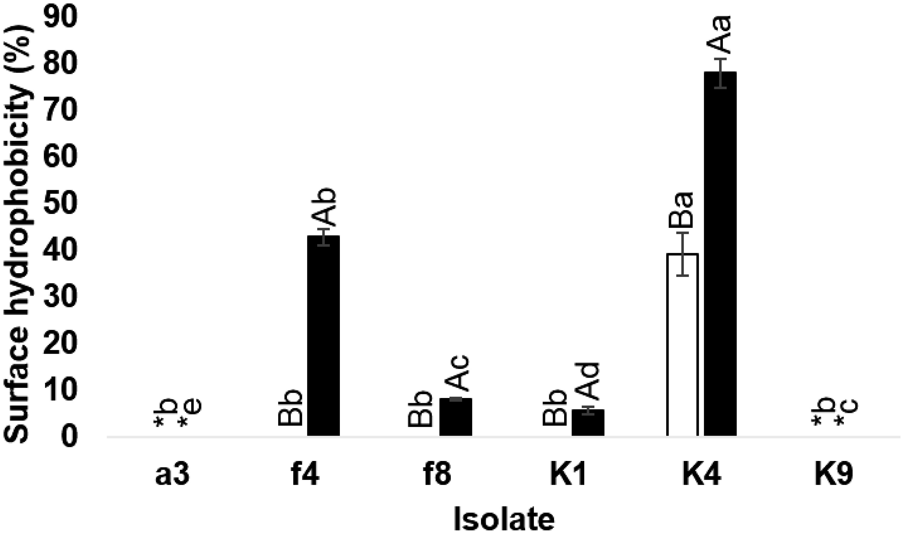
The probiotic potential of lactic acid bacteria (LAB) isolated from Thai traditional fermented food was investigated. Forty-two samples were collected from four markets in Phra Nakhon Si Ayutthaya Province. Out of 50 isolated LAB, 6 (a3, f4, f8, K1, K4 and K9) obtained from pla-ra and bamboo shoot pickle samples showed high tolerance to gastrointestinal tract conditions. These isolates were selected to identify and characterize their probiotic properties. Isolate a3 was identified as Weissella thailandensis, isolates f4 and f8 were identified as belonging to Enterococcus thailandicus and isolates K1, K4 and K9 were determined as Limosilactobacillus fermentum. All six LAB exhibited high autoaggregation ability (93.40–95.01%), while W. thailandensis isolate a3 showed potential for coaggregation in almost all the pathogenic bacteria tested. Cell-free supernatant (CFS) obtained from all isolates did not inhibit Staphylococcus aureus. CFS derived from L. fermentum isolate K4 showed the most efficient antimicrobial activity, in particular against Gram-negative bacteria, while L. fermentum isolate K4 presented high surface hydrophobicity in the presence of xylene and n-hexane. All LAB isolates were found to be resistant to clindamycin and nalidixic acid, whereas E. thailandicus isolate f8 exhibited resistance to most of the antibiotics tested. L. fermentum isolate K4 showed promise as a suitable probiotic candidate for future applications in the food industry due to tolerance to gastrointestinal tract conditions with high surface hydrophobicity and inhibited most of the pathogens tested.
Citation: Sunisa Suwannaphan. Isolation, identification and potential probiotic characterization of lactic acid bacteria from Thai traditional fermented food[J]. AIMS Microbiology, 2021, 7(4): 431-446. doi: 10.3934/microbiol.2021026
The probiotic potential of lactic acid bacteria (LAB) isolated from Thai traditional fermented food was investigated. Forty-two samples were collected from four markets in Phra Nakhon Si Ayutthaya Province. Out of 50 isolated LAB, 6 (a3, f4, f8, K1, K4 and K9) obtained from pla-ra and bamboo shoot pickle samples showed high tolerance to gastrointestinal tract conditions. These isolates were selected to identify and characterize their probiotic properties. Isolate a3 was identified as Weissella thailandensis, isolates f4 and f8 were identified as belonging to Enterococcus thailandicus and isolates K1, K4 and K9 were determined as Limosilactobacillus fermentum. All six LAB exhibited high autoaggregation ability (93.40–95.01%), while W. thailandensis isolate a3 showed potential for coaggregation in almost all the pathogenic bacteria tested. Cell-free supernatant (CFS) obtained from all isolates did not inhibit Staphylococcus aureus. CFS derived from L. fermentum isolate K4 showed the most efficient antimicrobial activity, in particular against Gram-negative bacteria, while L. fermentum isolate K4 presented high surface hydrophobicity in the presence of xylene and n-hexane. All LAB isolates were found to be resistant to clindamycin and nalidixic acid, whereas E. thailandicus isolate f8 exhibited resistance to most of the antibiotics tested. L. fermentum isolate K4 showed promise as a suitable probiotic candidate for future applications in the food industry due to tolerance to gastrointestinal tract conditions with high surface hydrophobicity and inhibited most of the pathogens tested.

| [1] | Fontana L, Bermudez-Brito M, Plaza-Diaz J, et al. (2013) Sources, isolation, characterization and evaluation of probiotics. Br J Nutr 109: 35-50. |
| [2] | Hartayanie L, Lindayani, Murniati MP (2016) Antimicrobial activity of Lactic acid bacteria from bamboo shoot pickles fermented at 15 °C. Microbiol Indones 10: 71-77. |
| [3] | Ayyash M, Liu SQ, Mheiri AA, et al. (2019) In vitro investigation of health-promoting benefits of fermented camel sausage by novel probiotic Lactobacillus plantarum: A comparative study with beef sausage. LWT-Food Sci Technol 99: 346-354. |
| [4] | Yongsmith B, Malaphan W (2016) Traditional Fermented Foods in Thailand. Traditional Foods New York: Springer Science+Business Media, 31-58. |
| [5] | FAO/WHO FAO/WHO working group report on drafting guidelines for the evaluation of probiotics in food, London, Ontario, Canada, April 30 and May 1, World Health Organization (2002) .Available from: https://www.who.int/foodsafety/\fs_management/en/probiotic_guidelines.pdf. |
| [6] | Abulfazl B (2012) Isolation and molecular study of potentially probiotic lactobacilli in traditional white cheese of Tabriz in iran. Ann Biol Res 3: 2213-2216. |
| [7] | Arshad FA, Mehmood R, Hussain S (2018) Lactobacilli as probiotics and their isolation from different sources. Br J Res 5: 1-11. |
| [8] | Gibson GR, Hutkins R, Sanders ME, et al. (2017) The International scientific association for probiotics and prebiotics (ISAPP) consensus statement on the definition and scope of prebiotics. Expert Consensus Statement 14: 491-502. |
| [9] | Musikasang H, Tani A, H-kittikun A, et al. (2009) Probiotic potential of lactic acid bacteria isolated from chicken gastrointestinal digestive tract. World J Microbiol Biotechnol 25: 1337-1345. |
| [10] | Ranadheera RDCS, Baines SK, Adams MC (2010) Importance of food in probiotic efficacy. Food Res Int 43: 1-7. |
| [11] | Sivamaruthi BS, Kesika P, Chaiyasut C (2018) Thai fermented foods as a versatile source of bioactive microorganisms-A comprehensive review. Sci Pharm 86: 2-11. |
| [12] | Yadav R (2017) Probiotics for Human Health. Current Progress and Applications. Recent advances in Applied Microbiology Singapore: Springer, 133-147. |
| [13] | Soccol CR, Vandenberghe LPDS, Spier MR, et al. (2010) The potential of probiotics: A review. Food Technol Biotechnol 48: 413-434. |
| [14] | Hoque MZ, Akter F, Hossain KM, et al. (2010) Isolation, identification and analysis of probiotic properties of Lactobacillus spp. From selective regional yoghurts. World J Dairy Food Sci 5: 39-46. |
| [15] | Arboleya S, Ruas-Madiedo P, Margolles A, et al. (2011) Characterization and in vitro properties of potentially probiotic Bifidobacterium strains isolated from breast-milk. Int J Food Microbiol 149: 28-36. |
| [16] | Re BD, Sgorbati B, Miglioli M, et al. (2000) Adhesion, autoaggregation and hydrophobicity of 13 strains of Bifidobacterium longum. Lett Appl Microbiol 31: 438-442. |
| [17] | Guan C, Chen X, Jiang X, et al. (2020) In vitro studies of adhesion properties of six lactic acid bacteria isolated from the longevous population of China. RSC Adv 10: 24234-24240. |
| [18] | Tagg JR, McGiven AR (1971) Assay system for bacteriocins. Appl Microbiol 21: 943. |
| [19] | Charteris WP, Kelly PM, Morelli L, et al. (1998) Antibiotic susceptibility of potentially probiotic Lactobacillus species. J Food Prot 61: 1636-1643. |
| [20] | Miyashita M, Yukphan P, Chaipitakchonlatarn W, et al. (2012) 16S rRNA gene sequence analysis of lactic acid bacteria isolated from fermented foods in Thailand. Microbiol Cult Coll 28: 1-9. |
| [21] | Rodpai R, Sanpool O, Thanchomnang, et al. (2021) Investigating the microbiota of fermented fish products (Pla-ra) from different communities of northeastern Thailand. PLos One 16: e0245227. |
| [22] | Thakur K, Rajani CS, Kumar S, et al. (2016) Fermented bamboo shoots: a riche niche for beneficial microbes. J Bacteriol Mycol 2: 87-93. |
| [23] | Lindayani L, Hartayanie L, Murniati MP (2018) Probiotic potential of lactic acid bacteria from yellow bamboo shoot fermentation using 2.5% and 5% brine at room temperature. Microbiol Indones 12: 30-34. |
| [24] | Mir SA, Raja J, Masoodi FA (2018) Fermented vegetables, a rich repository of beneficial probiotics-a review. Ferment Technol 7: 1-6. |
| [25] | Ben SR, Trabelsi I, Ben MR, et al. (2012) A new Lactobacillus plantarum strain, TN8, from the gastro intestinal tract of poultry induces high cytokine production. Anaerobe 18: 436-444. |
| [26] | Tanasupawat S, Shida O, Okada S, et al. (2000) Lactobacillus acidipiscis sp. nov. and Weissella thailandensis sp. nov., isolated from fermented fish in Thailand. Int J Syst Evol 50: 1479-1485. |
| [27] | Tanasupawat S, Sukontasing S, Lee JS (2008) Enterococcus thailandicus sp. nov., isolated from fermented sausage (‘mum’) in Thailand. Int J Syst Evol 58: 1630-1634. |
| [28] | Chen YS, Wu HC, Liu CH, et al. (2010) Isolation and characterization of lactic acid bacteria from jiang-sun (fermented bamboo shoots), a traditional fermented food in Taiwan. J Sci Food Agric 90: 1977-1982. |
| [29] | Behera P, Balaji S (2021) Health benefits of fermented bamboo shoots: The twenty-first century green gold of northeast India. Appl Biochem Biotechnol 193: 1800-1802. |
| [30] | Haghshenas B, Nami Y, Almasi A, et al. (2017) Isolation and characterization of probiotics from dairies. Iran J Microbiol 9: 234-243. |
| [31] | Abrunhosa L, Inês A, Rodrigues AI, et al. (2014) Biodegradation of ochratoxin A by Pediococcus parvulus isolated from Douro wines. Int J Food Microbiol 188: 45-52. |
| [32] | Roghmann MC, McGrail L (2006) Novel ways of preventing antibiotic-resistant infections: What might the future hold? Am J Infect Control 34: 469-475. |
| [33] | Alkalbani NS, Turner MS, Ayyash MM (2019) Isolation, identification, and potential probiotic characterization of isolated lactic acid bacteria and in vitro investigation of cytotoxicity, antioxidant, and antidiabetic activities in fermented sausage. Microb Cell Fact 18: 3-12. |
| [34] | Pessoa WFB, Melgaco ACC, de Almeida ME, et al. (2017) In vitro activity of Lactobacilli with probiotic potential isolated from cocoa fermentation against Gardnerella vaginalis. Biomed Res Int 2017: 1-10. |
| [35] | Trunk T, Khalil HS, Leo JC (2018) Bacterial autoaggregation. Microbiology 4: 140-164. |
| [36] | Tuo Y, Yu H, Ai L, et al. (2013) Aggregation and adhesion properties of 22 Lactobacillus strains. J Dairy Sci 96: 4252-4257. |
| [37] | Kocabay S, Çetinkaya S (2020) Probiotic properties of a Lactobacillus fermentum isolated from new-born faeces. J Oleo Sci 69: 1579-1584. |
| [38] | Tamang B, Tamang JP (2009) Lactic acid bacteria isolated from indigenous fermented bamboo products of Arunachal Pradesh in India and their functionality. Food Biotechnol 23: 133-147. |
| [39] | He X, Lux R, Kuramitsu HK, et al. (2009) Achieving probiotic effects via modulating oral microbial ecology. Adv Dent Res 21: 53-56. |
| [40] | Santos KMO, Vieira ADS, Salles HO, et al. (2015) Safety, beneficial and technological properties of Enterococcus faecium isolated from Brazilian cheeses. Braz J Microbiol 46: 237-249. |
| [41] | Xiong L, Ni X, Niu L, et al. (2019) Isolation and preliminary screening of a Weissella confusa strain from giant panda (Ailuropoda melanoleuca). Probiotics Antimicrob Proteins 11: 535-544. |
| [42] | Zeng Y, Li Y, Wu QP, et al. (2020) Evaluation of the antibacterial activity and probiotic potential of Lactobacillus plantarum isolated from Chinese homemade pickles. Can J Infect Dis Med Microbiol 2020: 1-11. |
| [43] | Powthong P, Suntornthicharoen P (2015) Isolation, identification and analysis of probiotic properties of lactic acid bacteria from selective various traditional Thai fermented food and kefir. Pak J Nutr 14: 67-74. |
| [44] | Kamboj K, Vasquez A, Balada-Liasat JM (2015) Identification and significance of Weissella species infections. Front Microbiol 6: 1-7. |
| [45] | Wu Z, Wu B, Li Y, et al. (2021) Identification and safety assessment of Enterococcus thailandicus TC1 isolated from healthy pigs. PLoS One 16: e0254081. |
| [46] | EgervÄrn M, Danielsen M, Roos F, et al. (2007) Antibiotic susceptibility profiles of Lactobacillus reuteri and Lactobacillus fermentum. J Food Prot 70: 412-418. |
Figures(1) / Tables(6)

Sunisa Suwannaphan. Isolation, identification and potential probiotic characterization of lactic acid bacteria from Thai traditional fermented food[J]. AIMS Microbiology, 2021, 7(4): 431-446. doi: 10.3934/microbiol.2021026


 DownLoad: