
Citation: Kamila Tomoko Yuyama, Thaís Souto Paula da Costa Neves, Marina Torquato Memória, Iago Toledo Tartuci, Wolf-Rainer Abraham. Aurantiogliocladin inhibits biofilm formation at subtoxic concentrations[J]. AIMS Microbiology, 2017, 3(1): 50-60. doi: 10.3934/microbiol.2017.1.50
[1] | Joseph L. Shomberg . Well-posedness and global attractors for a non-isothermal viscous relaxationof nonlocal Cahn-Hilliard equations. AIMS Mathematics, 2016, 1(2): 102-136. doi: 10.3934/Math.2016.2.102 |
[2] | Jianxia He, Ming Li . Existence of global solution to 3D density-dependent incompressible Navier-Stokes equations. AIMS Mathematics, 2024, 9(3): 7728-7750. doi: 10.3934/math.2024375 |
[3] | Geetika Saini, B. N. Hanumagowda, S. V. K. Varma, Jasgurpreet Singh Chohan, Nehad Ali Shah, Yongseok Jeon . Impact of couple stress and variable viscosity on heat transfer and flow between two parallel plates in conducting field. AIMS Mathematics, 2023, 8(7): 16773-16789. doi: 10.3934/math.2023858 |
[4] | Adel M. Al-Mahdi, Maher Noor, Mohammed M. Al-Gharabli, Baowei Feng, Abdelaziz Soufyane . Stability analysis for a Rao-Nakra sandwich beam equation with time-varying weights and frictional dampings. AIMS Mathematics, 2024, 9(5): 12570-12587. doi: 10.3934/math.2024615 |
[5] | Zayd Hajjej . A suspension bridges with a fractional time delay: Asymptotic behavior and Blow-up in finite time. AIMS Mathematics, 2024, 9(8): 22022-22040. doi: 10.3934/math.20241070 |
[6] | S. R. Mishra, Subhajit Panda, Mansoor Alshehri, Nehad Ali Shah, Jae Dong Chung . Sensitivity analysis on optimizing heat transfer rate in hybrid nanofluid flow over a permeable surface for the power law heat flux model: Response surface methodology with ANOVA test. AIMS Mathematics, 2024, 9(5): 12700-12725. doi: 10.3934/math.2024621 |
[7] | Zhongying Liu, Yang Liu, Yiqi Jiang . Global solvability of 3D non-isothermal incompressible nematic liquid crystal flows. AIMS Mathematics, 2022, 7(7): 12536-12565. doi: 10.3934/math.2022695 |
[8] | Mingyu Zhang . On the Cauchy problem of 3D nonhomogeneous micropolar fluids with density-dependent viscosity. AIMS Mathematics, 2024, 9(9): 23313-23330. doi: 10.3934/math.20241133 |
[9] | Takumi Washio, Akihiro Fujii, Toshiaki Hisada . On random force correction for large time steps in semi-implicitly discretized overdamped Langevin equations. AIMS Mathematics, 2024, 9(8): 20793-20810. doi: 10.3934/math.20241011 |
[10] | Said Mesloub, Hassan Altayeb Gadain, Lotfi Kasmi . On the well posedness of a mathematical model for a singular nonlinear fractional pseudo-hyperbolic system with nonlocal boundary conditions and frictional damping terms. AIMS Mathematics, 2024, 9(2): 2964-2992. doi: 10.3934/math.2024146 |
The nonsingular H-matrix and its subclass play an important role in a lot of fields of science such as computational mathematics, mathematical physics, and control theory, see [1,2,3,4]. Meanwhile, the infinity norm bounds of the inverse for nonsingular H-matrices can be used in convergence analysis of matrix splitting and matrix multi-splitting iterative methods for solving large sparse systems of linear equations [5], as well as bounding errors of linear complementarity problems [6,7]. In recent years, many scholars have developed a deep research interest in the infinity norm of the inverse for special nonsingular H-matrices, such as GSDD1 matrices [8], CKV-type matrices [9], S-SDDS matrices [10], S-Nekrasov matrices [11], S-SDD matrices [12], and so on, which depends only on the entries of the matrix.
In this paper, we prove that M is a nonsingular H-matrix by constructing a scaling matrix D for SDD+1 matrices such that MD is a strictly diagonally dominant matrix. The use of the scaling matrix is important for some applications, for example, the infinity norm bound of the inverse [13], eigenvalue localization [3], and error bounds of the linear complementarity problem [14]. We consider the infinity norm bound of the inverse for the SDD+1 matrix by multiplying the scaling matrix, then we use the result to discuss the error bounds of the linear complementarity problem.
For a positive integer n≥2, let N denote the set {1,2,…,n} and Cn×n(Rn×n) denote the set of all complex (real) matrices. Successively, we review some special subclasses of nonsingular H-matrices and related lemmas.
Definition 1. [5] A matrix M=(mij)∈Cn×n is called a strictly diagonally dominant (SDD) matrix if
|mii|>ri(M),∀i∈N, | (1.1) |
where ri(M)=n∑j=1,j≠i|mij|.
Various generalizations of SDD matrices have been introduced and studied in the literatures, see [7,15,16,17,18].
Definition 2. [8] A matrix M=(mij)∈Cn×n is called a generalized SDD1 (GSDD1) matrix if
{ri(M)−pN2i(M)>0,i∈N2,(ri(M)−pN2i(M))(|mjj|−pN1j(M))>pN1i(M)pN2j(M),i∈N2,j∈N1, | (1.2) |
where N1={i∈N|0<|mii|≤ri(M)}, N2={i∈N||mii|>ri(M)}, pN2i(M)=∑j∈N2∖{i}|mij|rj(M)|mjj|, pN1i(M)=∑j∈N1∖{i}|mij|,i∈N.
Definition 3. [9] A matrix M=(mij)∈Cn×n, with n⩾2, is called a CKV-type matrix if for all i∈N the set S⋆i(M) is not empty, where
S⋆i(M)={S∈∑(i):|mii|>rsi(M),andforallj∈¯S(|mii|−rSi(M))(|mjj|−r¯Sj(M))>r¯Si(M)rSj(M)}, |
with ∑(i)={S⊊N:i∈S} and rSi(M):=∑j∈S∖{i}|mij|.
Lemma 1. [8] Let M=(mij)∈Cn×n be a GSDD1 matrix. Then
‖M−1‖∞≤max{ε,maxi∈N2ri(M)|mii|}min{mini∈N2ϕi,mini∈N1ψi}, | (1.3) |
where
ϕi=ri(M)−∑j∈N2∖{i}|mij|rj(M)|mjj|−∑j∈N1|mij|ε,i∈N2, | (1.4) |
ψi=|mii|ε−∑j∈N1∖{i}|mij|ε−∑j∈N2|mij|rj(M)|mjj|,i∈N1, | (1.5) |
and
ε∈{maxi∈N1pN2i(M)|mii|−pN1i(M),minj∈N2rj(M)−pN2j(M)pN1j(M)}. | (1.6) |
Lemma 2. [8] Suppose that M=(mij)∈Rn×n is a GSDD1 matrix with positive diagonal entries, and D=diag(di) with di∈[0,1]. Then
maxd∈[0,1]n‖(I−D+DM)−1‖∞≤max{max{ε,maxi∈N2ri(M)|mii|}min{mini∈N2ϕi,mini∈N1ψi},max{ε,maxi∈N2ri(M)|mii|}min{ε,mini∈N2ri(M)|mii|}}, | (1.7) |
where ϕi,ψi,andε are shown in (1.4)–(1.6), respectively.
Definition 4. [19] Matrix M=(mij)∈Cn×n is called an SDD1 matrix if
|mii|>ri′(M),foreachi∈N1, | (1.8) |
where
ri′(M)=∑j∈N1∖{i}|mij|+∑j∈N2∖{i}|mij|rj(M)|mjj|, |
N1={i∈N|0<|mii|≤ri(M)},N2={i∈N||mii|>ri(M)}. |
The rest of this paper is organized as follows: In Section 2, we propose a new subclass of nonsingular H-matrices referred to SDD+1 matrices, discuss some of the properties of it, and consider the relationships among subclasses of nonsingular H-matrices by numerical examples, including SDD1 matrices, GSDD1 matrices, and CKV-type matrices. At the same time, a scaling matrix D is constructed to verify that the matrix M is a nonsingular H-matrix. In Section 3, two methods are utilized to derive two different upper bounds of infinity norm for the inverse of the matrix (one with parameter and one without parameter), and numerical examples are used to show the validity of the results. In Section 4, two error bounds of the linear complementarity problems for SDD+1 matrices are given by using the scaling matrix D, and numerical examples are used to illustrate the effectiveness of the obtained results. Finally, a summary of the paper is given in Section. 5.
For the sake of the following description, some symbols are first explained:
N=N1∪N2,N1=N(1)1∪N(1)2≠∅,ri(M)≠0,N1={i∈N|0<|mii|≤ri(M)},N2={i∈N||mii|>ri(M)}, | (2.1) |
N(1)1={i∈N1|0<|mii|≤ri′(M)},N(1)2={i∈N1||mii|>ri′(M)}, | (2.2) |
ri′(M)=∑j∈N1∖{i}|mij|+∑j∈N2|mij|rj(M)|mjj|,i∈N1. | (2.3) |
By the definitions of N(1)1 and N(1)2, for N1=N(1)1∪N(1)2, ri′(M) in Definition 4 can be rewritten as
ri′(M)=∑j∈N1∖{i}|mij|+∑j∈N2∖{i}|mij|rj(M)|mjj|=∑j∈N(1)1∖{i}|mij|+∑j∈N(1)2∖{i}|mij|+∑j∈N2∖{i}|mij|rj(M)|mjj|. | (2.4) |
According to (2.4), it is easy to get the following equivalent form for SDD1 matrices.
A matrix M is called an SDD1 matrix, if
{|mii|>∑j∈N(1)1∖{i}|mij|+∑j∈N(1)2|mij|+∑j∈N2rj(M)|mjj||mij|,i∈N(1)1,|mii|>∑j∈N(1)1|mij|+∑j∈N(1)2∖{i}|mij|+∑j∈N2rj(M)|mjj||mij|,i∈N(1)2. | (2.5) |
By scaling conditions (2.5), we introduce a new class of matrices. As we will see, these matrices belong to a new subclass of nonsingular H-matrices.
Definition 5. A matrix M=(mij)∈Cn×n is called an SDD+1 matrix if
{|mii|>Fi(M)=∑j∈N(1)1∖{i}|mij|+∑j∈N(1)2|mij|r′j(M)|mjj|+∑j∈N2|mij|rj(M)|mjj|,i∈N(1)1,|mii|>F′i(M)=∑j∈N(1)2∖{i}|mij|+∑j∈N2|mij|,i∈N(1)2, | (2.6) |
where N1,N2,N(1)1,N(1)2,andri′(M) are defined by (2.1)–(2.3), respectively.
Proposition 1. If M=(mij)∈Cn×n is an SDD+1 matrix and N(1)1≠∅, then ∑j∈N(1)2|mij|+∑j∈N2|mij|≠0 for i∈N(1)1.
Proof. Assume that there exists i∈N(1)1 such that ∑j∈N(1)2|mij|+∑j∈N2|mij|=0. We find that
|mii|>∑j∈N(1)1∖{i}|mij|=∑j∈N(1)1∖{i}|mij|+∑j∈N(1)2∖{i}|mij|+∑j∈N2|mij|rj(M)|mjj|=∑j∈N(1)1∖{i}|mij|+∑j∈N2|mij|rj(M)|mjj|=r′i(M), |
which contradicts i∈N(1)1. The proof is completed.
Proposition 2. If M=(mij)∈Cn×n is an SDD+1 matrix with N(1)2=∅, then M is also an SDD1 matrix.
Proof. From Definition 5, we have
|mii|>∑j∈N(1)1∖{i}|mij|+∑j∈N2|mij|rj(M)|mjj|,∀i∈N(1)1. |
Because of N1=N(1)1, it holds that
|mii|>∑j∈N1∖{i}|mij|+∑j∈N2|mij|rj(M)|mjj|=ri′(M),∀i∈N1. |
The proof is completed.
Example 1. Consider the following matrix:
M1=(8−52339624−290−31210). |
In fact, N1={1,2} and N2={3,4}. Through calculations, we obtain that
r1(M1)=10,r2(M1)=11,r3(M1)=6,r4(M1)=6, |
r1′(M1)=|m12|+|m13|r3(M1)|m33|+|m14|r4(M1)|m44|≈8.1333, |
r2′(M1)=|m21|+|m23|r3(M1)|m33|+|m24|r4(M1)|m44|=8.2000. |
Because of |m11|=8<8.1333=r1′(M1), M1 is not an SDD1 matrix.
Since
r′1(M1)≈8.1333>|m11|=8, |
r′2(M1)=8.2000<|m22|=9, |
then N(1)1={1}, N(1)2={2}. As
|m11|=8>|m12|r′2(M1)|m22|+|m13|r3(M1)|m33|+|m14|r4(M1)|m44|≈7.6889, |
|m22|=9>|m23|+|m24|=8, |
M1 is an SDD+1 matrix by Definition 5.
Example 2. Consider the following matrix:
M2=(1548−77−51−216). |
In fact, N1={2} and N2={1,3}. By calculations, we get
r1(M2)=12,r2(M2)=12,r3(M2)=3, |
r2′(M2)=0+|m21|r1(M2)|m11|+|m23|r3(M2)|m33|=6.5375. |
Because of |m22|=7>6.5375=r2′(M2), M2 is an SDD1 matrix.
According to
r′2(M2)=6.5375<|m22|=7, |
we know that N(1)2={2}. In addition,
|m22|=7<0+|m21|+|m23|=12, |
and M2 is not an SDD+1 matrix.
As shown in Examples 1 and 2 and Proposition 2, it can be seen that SDD+1 matrices and SDD1 matrices have an intersecting relationship:
{SDD1}⊈{SDD+1} and {SDD+1}⊈{SDD1}. |
The following examples will demonstrate the relationships between SDD+1 matrices and other subclasses of nonsingular H-matrices.
Example 3. Consider the following matrix:
M3=(401−2120104.14620−2334804−620230−42040). |
In fact, N1={2,3} and N2={1,4,5}. Through calculations, we get that
r1(M3)=6,r2(M3)=14.1,r3(M3)=34,r4(M3)=12,r5(M3)=36, |
r′2(M3)=|m23|+|m21|r1(M3)|m11|+|m24|r4(M3)|m44|+|m25|r5(M3)|m55|=11.9>|m22|, |
r′3(M3)=|m32|+|m31|r1(M3)|m11|+|m34|r4(M3)|m44|+|m35|r5(M3)|m55|=14.6<|m33|, |
and N(1)1={2}, N(1)2={3}. Because of
|m22|>|m23|r′3(M3)|m33|+|m21|r1(M3)|m11|+|m24|r4(M3)|m44|+|m25|r5(M3)|m55|≈9.61, |
|m33|=33>0+|m31|+|m34|+|m35|=32. |
So, M3 is an SDD+1 matrix. However, since |m22|=10<11.9=r′2(M3), then M3 is not an SDD1 matrix. And we have
pN11(M3)=3,pN12(M3)=4.1,pN13(M3)=2,pN14(M3)=10,pN15(M3)=6, |
pN21(M3)=2.4,pN22(M3)=7.8,pN23(M3)=12.6,pN24(M3)=1.8,pN25(M3)=4.5. |
Note that, taking i=1,j=2, we have that
(r1(M3)−pN21(M3))(|m22|−pN12(M3))=21.24<pN11(M3)pN22(M3)=23.4. |
So, M3 is not a GSDD1 matrix. Moreover, it can be verified that M3 is not a CKV-type matrix.
Example 4. Consider the following matrix:
M4=(−10.4000.5100−12.11−0.51−20.311). |
It is easy to check that M4 is a CKV-type matrix and a GSDD1 matrix, but not an SDD+1 matrix.
Example 5. Consider the following matrix:
M5=(30.78666.755.256362.2533.78361.54.532.256633.036665.2530.752.25628.531.52.254.54.50.755.251.50.7529.28662.255.254.51.50.755.2535.2835.255.2534.5636.7530.033.754.50.753.757.55.250.750.7529.28). |
We know that M5 is not only an SDD+1 matrix, but also CKV-type matrix and GSDD1 matrix.
According to Examples 3–5, we find that SDD+1 matrices have intersecting relationships with the CKV-type matrices and GSDD1 matrices, as shown in the Figure 1 below. In this paper, we take N1≠∅ and ri(M)≠0, so we will not discuss the relationships among SDD matrices, SDD+1 matrices, and GSDD1 matrices.
Example 6. Consider the tri-diagonal matrix M∈Rn×n arising from the finite difference method for free boundary problems [8], where
M6=(b+αsin(1n)c0⋯0ab+αsin(2n)c⋯0⋱⋱⋱0⋯ab+αsin(n−1n)c0⋯0ab+αsin(1)). |
Take n=12000, a=5.5888, b=16.5150, c=10.9311, and α=14.3417. It is easy to verify that M6 is an SDD+1 matrix, but not an SDD matrix, a GSDD1 matrix, an SDD1 matrix, nor a CKV-type matrix.
As is shown in [19] and [8], SDD1 matrix and GSDD1 matrix are both nonsingular H-matrices, and there exists an explicit construction of the diagonal matrix D, whose diagonal entries are all positive, such that MD is an SDD matrix. In the following, we construct a positive diagonal matrix D involved with a parameter that scales an SDD+1 matrix to transform it into an SDD matrix.
Theorem 1. Let M=(mij)∈Cn×n be an SDD+1 matrix. Then, there exists a diagonal matrix D=diag(d1,d2,⋯,dn) with
di={1,i∈N(1)1,ε+r′i(M)|mii|,i∈N(1)2,ε+ri(M)|mii|,i∈N2, | (2.7) |
where
0<ε<mini∈N(1)1pi, | (2.8) |
and for all i∈N(1)1, we have
pi=|mii|−∑j∈N(1)1∖{i}|mij|−∑j∈N(1)2|mij|r′j(M)|mjj|−∑j∈N2|mij|rj(M)|mjj|∑j∈N(1)2|mij|+∑j∈N2|mij|, | (2.9) |
such that MD is an SDD matrix.
Proof. By (2.6), we have
|mii|−∑j∈N(1)1∖{i}|mij|−∑j∈N(1)2|mij|r′j(M)|mjj|−∑j∈N2|mij|rj(M)|mjj|>0. | (2.10) |
From Proposition 1, for all i∈N(1)1, it is easy to know that
pi=|mii|−∑j∈N(1)1∖{i}|mij|−∑j∈N(1)2|mij|r′j(M)|mjj|−∑j∈N2|mij|rj(M)|mjj|∑j∈N(1)2|mij|+∑j∈N2|mij|>0. | (2.11) |
Immediately, there exists a positive number ε such that
0<ε<mini∈N(1)1pi. | (2.12) |
Now, we construct a diagonal matrix D=diag(d1,d2,⋯,dn) with
di={1,i∈N(1)1,ε+r′i(M)|mii|,i∈N(1)2,ε+ri(M)|mii|,i∈N2, | (2.13) |
where ε is given by (2.12). It is easy to find that all the elements in the diagonal matrix D are positive. Next, we will prove that MD is strictly diagonally dominant.
Case 1. For each i∈N(1)1, it is not difficult to find that |(MD)ii|=|mii|. By (2.11) and (2.13), we have
ri(MD)=∑j∈N(1)1∖{i}dj|mij|+∑j∈N(1)2dj|mij|+∑j∈N2dj|mij|=∑j∈N(1)1∖{i}|mij|+∑j∈N(1)2(ε+r′j(M)|mjj|)|mij|+∑j∈N2(ε+rj(M)|mjj|)|mij|=∑j∈N(1)1∖{i}|mij|+∑j∈N(1)2|mij|r′j(M)|mjj|+∑j∈N2|mij|rj(M)|mjj|+ε(∑j∈N(1)2|mij|+∑j∈N2|mij|)<|mii|=|(MD)ii|. |
Case 2. For each i∈N(1)2, we obtain
|(MD)ii|=|mii|(ε+r′i(M)|mii|)=ε|mii|+r′i(M). | (2.14) |
From (2.3), (2.13), and (2.14), we derive that
ri(MD)=∑j∈N(1)1|mij|+∑j∈N(1)2∖{i}|mij|r′j(M)|mjj|+∑j∈N2|mij|rj(M)|mjj|+ε(∑j∈N(1)2∖{i}|mij|+∑j∈N2|mij|)≤r′i(M)+ε(∑j∈N(1)2∖{i}|mij|+∑j∈N2|mij|)<r′i(M)+ε|mii|=|(MD)ii|. |
The first inequality holds because of |mii|>r′i(M) for any i∈N(1)2, and
r′i(M)=∑j∈N1∖{i}|mij|+∑j∈N2|mij|rj(M)|mjj|=∑j∈N(1)1|mij|+∑j∈N(1)2∖{i}|mij|+∑j∈N2|mij|rj(M)|mjj|≥∑j∈N(1)1|mij|+∑j∈N(1)2∖{i}|mij|r′j(M)|mjj|+∑j∈N2|mij|rj(M)|mjj|. |
Case 3. For each i∈N2, we have
ri(M)=∑j∈N1∖{i}|mij|+∑j∈N2∖{i}|mij|=∑j∈N(1)1|mij|+∑j∈N(1)2|mij|+∑j∈N2∖{i}|mij|≥∑j∈N(1)1|mij|+∑j∈N(1)2|mij|r′j(M)|mjj|+∑j∈N2∖{i}|mij|rj(M)|mjj|. | (2.15) |
Meanwhile, for each i∈N2, it is easy to get
|mii|>ri(M)≥∑j∈N(1)2|mij|+∑j∈N2∖{i}|mij|, | (2.16) |
and
|(MD)ii|=|mii|(ε+ri(M)|mii|)=ε|mii|+ri(M). | (2.17) |
From (2.13), (2.15), and (2.16), it can be deduced that
ri(MD)=∑j∈N(1)1|mij|+∑j∈N(1)2(ε+r′j(M)|mjj|)|mij|+∑j∈N2∖{i}(ε+rj(M)|mjj|)|mij|=∑j∈N(1)1|mij|+∑j∈N(1)2|mij|r′j(M)|mjj|+∑j∈N2∖{i}|mij|rj(M)|mjj|+ε(∑j∈N(1)2|mij|+∑j∈N2∖{i}|mij|)<ri(M)+ε|mii|=|(MD)ii|. |
So, |(MD)ii|>ri(MD) for i∈N. Thus, MD is an SDD matrix. The proof is completed.
It is well known that the H-matrix M is nonsingular if there exists a diagonal matrix D such that MD is an SDD matrix (see [1,19]). Therefore, from Theorem 1, SDD+1 matrices are nonsingular H-matrices.
Corollary 1. Let M=(mij)∈Cn×n be an SDD+1 matrix. Then, M is also an H-matrix. If, in addition, M has positive diagonal entries, then det(M)>0.
Proof. We see from Theorem 1 that there is a positive diagonal matrix D such that MD is an SDD matrix (cf. (M35) of Theorem 2.3 of Chapter 6 of [1]). Thus, M is a nonsingular H-matrix. Since the diagonal entries of M and D are positive, MD has positive diagonal entries. From the fact that MD is an SDD matrix, it is well known that 0<det(MD)=det(M)det(D), which means det(M)>0.
In this section, we start to consider two infinity norm bounds of the inverse of SDD+1 matrices. Before that, some notations are defined:
Mi=|mii|−∑j∈N(1)1∖{i}|mij|−∑j∈N(1)2|mij|r′j(M)|mjj|−∑j∈N2|mij|rj(M)|mjj|−ε(∑j∈N(1)2|mij|+∑j∈N2|mij|),i∈N(1)1, | (3.1) |
Ni=r′i(M)−∑j∈N(1)1|mij|−∑j∈N(1)2∖{i}|mij|r′j(M)|mjj|−∑j∈N2|mij|rj(M)|mjj|+ε(|mii|−∑j∈N(1)2∖{i}|mij|−∑j∈N2|mij|),i∈N(1)2, | (3.2) |
Zi=ri(M)−∑j∈N(1)1|mij|−∑j∈N(1)2|mij|r′j(M)|mjj|−∑j∈N(1)2∖{i}|mij|rj(M)|mjj|+ε(|mii|−∑j∈N(1)2|mij|−∑j∈N2∖{i}|mij|),i∈N2. | (3.3) |
Next, let us review an important result proposed by Varah (1975).
Theorem 2. [20] If M=(mij)∈Cn×n is an SDD matrix, then
‖M−1‖∞≤1mini∈N{|mii|−ri(M)}. | (3.4) |
Theorem 2 can be used to bound the infinity norm of the inverse of an SDD matrix. This theorem together with the scaling matrix D=diag(d1,d2,⋯,dn) allows us to gain the following Theorem 3.
Theorem 3. Let M=(mij)∈Cn×n be an SDD+1 matrix. Then,
‖M−1‖∞≤max{1,maxi∈N(1)2(ε+r′i(M)|mii|),maxi∈N2(ε+ri(M)|mii|)}min{mini∈N(1)1Mi,mini∈N(1)2Ni,mini∈N2Zi}, | (3.5) |
where ε, Mi,Ni,andZi are defined in (2.8), (2.9), and (3.1)–(3.3), respectively.
Proof. By Theorem 1, there exists a positive diagonal matrix D such that MD is an SDD matrix, where D is defined as (2.13). Hence, we have the following result:
‖M−1‖∞=‖D(D−1M−1)‖∞=‖D(MD)−1‖∞≤‖D‖∞‖(MD)−1‖∞ | (3.6) |
and
‖D‖∞=max1≤i≤ndi=max{1,maxi∈N(1)2(ε+r′i(M)|mii|),maxi∈N2(ε+ri(M)|mii|)}, |
where ε is given by (2.8). Note that MD is an SDD matrix, by Theorem 2, we have
‖(MD)−1‖∞≤1mini∈N{|(MD)ii|−ri(MD)}. |
However, there are three scenarios to solve |(MD)ii|−ri(MD). For i∈N(1)1, we get
|(MD)ii|−ri(MD)=|mii|−∑j∈N(1)1∖{i}|mij|−∑j∈N(1)2(ε+r′j(M)|mjj|)|mij|−∑j∈N2(ε+rj(M)|mjj|)|mij|=|mii|−∑j∈N(1)1∖{i}|mij|−∑j∈N(1)2|mij|r′j(M)|mjj|−∑j∈N2|mij|rj(M)|mjj|−ε(∑j∈N(1)2|mij|+∑j∈N2|mij|)=Mi. |
For i∈N(1)2, we have
|(MD)ii|−ri(MD)=(ε+r′i(M)|mii|)|mii|−∑j∈N(1)1|mij|−∑j∈N(1)2∖{i}(ε+r′j(M)|mjj|)|mij|−∑j∈N2(ε+rj(M)|mjj|)|mij|=r′i(M)−∑j∈N(1)1|mij|−∑j∈N(1)2∖{i}|mij|r′j(M)|mjj|−∑j∈N2|mij|rj(M)|mjj|+ε(|mii|−∑j∈N(1)2∖{i}|mij|−∑j∈N2|mij|)=Ni. |
For i∈N2, we obtain
|(MD)ii|−ri(MD)=(ε+ri(M)|mii|)|mii|−∑j∈N(1)1|mij|−∑j∈N(1)2(ε+r′j(M)|mjj|)|mij|−∑j∈N2∖{i}(ε+rj(M)|mjj|)|mij|=ri(M)−∑j∈N(1)1|mij|−∑j∈N(1)2|mij|r′j(M)|mjj|−∑j∈N2∖{i}|mij|rj(M)|mjj|+ε(|mii|−∑j∈N(1)2|mij|−∑j∈N2∖{i}|mij|)=Zi. |
Hence, according to (3.6) we have
‖M−1‖∞≤max{1,maxi∈N(1)2(ε+r′i(M)|mii|),maxi∈N2(ε+ri(M)|mii|)}min{mini∈N(1)1Mi,mini∈N(1)2Ni,mini∈N2Zi}. |
The proof is completed.
It is noted that the upper bound in Theorem 3 is related to the interval values of the parameter. Next, another upper bound of ‖M−1‖∞ is given, which depends only on the elements in the matrix.
Theorem 4. Let M=(mij)∈Cn×n be an SDD+1 matrix. Then,
‖M−1‖∞≤max{1mini∈N(1)1{|mii|−Fi(M)},1mini∈N(1)2{|mii|−F′i(M)},1mini∈N2{|mii|−∑j≠i|mij|}}, | (3.7) |
where Fi(M) and F′i(M) are shown in (2.6).
Proof. By the well-known fact (see[21,22]) that
‖M−1‖−1∞=infx≠0‖Mx‖∞‖x‖∞=min‖x‖∞=1‖Mx‖∞=‖Mx‖∞=maxi∈N|(Mx)i|, | (3.8) |
for some x=[x1,x2,⋯,xn]T, we have
‖M−1‖−1∞≥|(Mx)i|. | (3.9) |
Assume that there is a unique k∈N such that ‖x‖∞=1=|xk|, then
mkkxk=(Mx)k−∑j≠kmkjxj=(Mx)k−∑j∈N(1)1∖{k}mkjxj−∑j∈N(1)2∖{k}mkjxj−∑j∈N2∖{k}mkjxj. |
When k∈N(1)1, let |xj|=r′j(M)|mjj| (j∈N(1)2), and |xj|=rj(M)|mjj| (j∈N2). Then we have
|mkk|=|mkkxk|=|(Mx)k−∑j∈N(1)1∖{k}mkjxj−∑j∈N(1)2mkjxj−∑j∈N2mkjxj|≤|(Mx)k|+|∑j∈N(1)1∖{k}mkjxj|+|∑j∈N(1)2mkjxj|+|∑j∈N2mkjxj|≤|(Mx)k|+∑j∈N(1)1∖{k}|mkj||xj|+∑j∈N(1)2|mkj||xj|+∑j∈N2|mkj||xj|≤|(Mx)k|+∑j∈N(1)1∖{k}|mkj|+∑j∈N(1)2|mkj|r′j(M)|mjj|+∑j∈N2|mkj|rj(M)|mjj|≤‖M−1‖−1∞+∑j∈N(1)1∖{k}|mkj|+∑j∈N(1)2|mkj|r′j(M)|mjj|+∑j∈N2|mkj|rj(M)|mjj|=‖M−1‖−1∞+Fk(M). |
Which implies that
‖M−1‖∞≤1|mkk|−Fk(M)≤1mini∈N(1)1{|mii|−Fi(M)}. |
For k∈N(1)2, let ∑j∈N(1)1|mkj|=0. It follows that
|mkk|≤|(Mx)k|+∑j∈N(1)1|mkj||xj|+∑j∈N(1)2∖{k}|mkj||xj|+∑j∈N2|mkj||xj|≤‖M−1‖−1∞+0+∑j∈N(1)2∖{k}|mkj|r′j(M)|mjj|+∑j∈N2|mkj|rj(M)|mjj|=‖M−1‖−1∞+F′k(M). |
Hence, we obtain that
‖M−1‖∞≤1|mkk|−F′k(M)≤1mini∈N(1)2{|mii|−F′i(M)}. |
For k∈N2, we get
0<mini∈N2{|mii|−∑j≠i|mij|}≤|mkk|−∑j≠k|mkj|, |
and
0<mini∈N2(|mii|−∑j≠i|mij|)|xk|≤|mkk||xk|−∑j≠k|mkj||xj|≤|mkk||xk|−|∑j≠kmkjxj|≤|∑k∈N2,j∈Nmkjxj|≤maxi∈N2|∑j∈Nmijxj|≤‖M−1‖−1∞, |
which implies that
‖M−1‖∞≤1|mkk|−Fk(M)≤1mini∈N2{|mii|−∑j≠i|mij|}. |
To sum up, we obtain that
‖M−1‖∞≤max{1mini∈N(1)1{|mii|−Fi(M)},1mini∈N(1)2{|mii|−F′i(M)},1mini∈N2{|mii|−∑j≠i|mij|}}. |
The proof is completed.
Next, some numerical examples are given to illustrate the superiority of our results.
Example 7. Consider the following matrix:
M7=(2−10000−12−10000−12−10000−12−10000−12−100002−1). |
It is easy to verify that M7 is an SDD+1 matrix. However, we know that M7 is not an SDD matrix, a GSDD1 matrix, an SDD1 matrix and a CKV-type matrix. By the bound in Theorem 3, we have
minpi=0.25,ε∈(0,0.25). |
When ε=0.1225, we get
‖M−17‖∞≤8.1633. |
The range of parameter values in Theorem 3 is not empty set, and its optimal solution can be illustrated through examples. In Example 7, the range of values for the error bound and its optimal solution can be seen from Figure 2. The bound for Example 7 is (8.1633,100), and the optimal solution for Example 7 is 8.1633.
However, according to Theorem 4, we obtain
‖M−17‖∞≤max{4,1,1}=4. |
Through this example, it can be found that the bound of Theorem 4 is better than Theorem 3 in some cases.
Example 8. Consider the following matrix:
M8=(b1c00000000ab2c00000000ab3c00000000ab4c00000000ab5c00000000ab6c00000000ab7c00000000ab8c00000000ab9c00000000ab10). |
Here, a=−2, c=2.99, b1=6.3304, b2=6.0833, b3=5.8412, b4=5.6065, b5=5.3814, b6=5.1684, b7=4.9695, b8=4.7866, b9=4.6217, and b10=4.4763. It is easy to verify that M8 is an SDD+1 matrix. However, we can get that M8 is not an SDD matrix, a GSDD1 matrix, an SDD1 matrix, and a CKV-type matrix. By the bound in Theorem 3, we have
minpi=0.1298,ε∈(0,0.1298). |
When ε=0.01, we have
‖M−18‖∞≤max{1,1.0002,0.9755}min{0.5981,0.0163,0.1765}=61.3620. |
If ε=0.1, we have
‖M−18‖∞≤max{1,1.0902,1.0655}min{0.1490,0.1632,0.1925}=7.3168. |
Taking ε=0.11, then it is easy to calculate
‖M−18‖∞≤max{1,1.1002,1.0755}min{0.0991,0.1795,0.1943}=11.1019. |
By the bound in Theorem 4, we have
‖M−18‖∞≤max{1.5433,0.6129,5.6054}=5.6054. |
Example 9. Consider the following matrix:
M9=(11.3−1.2−1.14.7−1.214.29.1−43.2−1.114.30.34.67.63.211.3). |
It is easy to verify that the matrix M9 is a GSDD1 matrix and an SDD+1 matrix. When M9 is a GSDD1 matrix, it can be calculated according to Lemma 1 that
ε∈(1.0484,1.1265). |
According to Figure 3, if we take ε=1.0964, we can obtain an optimal bound, namely
‖M−19‖∞≤6.1806. |
When M9 is an SDD+1 matrix, it can be calculated according to Theorem 3. We obtain
ε∈(0,0.2153). |
According to Figure 3, if we take ε=0.1707, we can obtain an optimal bound, namely
‖M−19‖∞≤1.5021. |
However, according to Theorem 4, we get
‖M−19‖∞≤max{0.3016,0.2564,0.2326}=0.3016. |
Example 10. Consider the following matrix:
M10=(7311173422933137). |
It is easy to verify that the matrix M10 is a CKV-type matrix and an SDD+1 matrix. When M10 is a CKV-type matrix, it can be calculated according to Theorem 21 in [9]
‖M10−1‖∞≤11. |
When M10 is an SDD+1matrix, take ε=0.0914 according to Theorem 3. We obtain an optimal bound, namely
‖M10−1‖∞≤max{1,0.8737,0.8692}min{0.0919,0.0914,3.5901}=10.9409. |
When M10 is an SDD+1matrix, it can be calculated according to Theorem 4. We can obtain
‖M10−1‖∞≤max{1,2149,1,1}=1.2149. |
From Examples 9 and 10, it is easy to know that the bound in Theorem 3 and Theorem 4 in our paper is better than available results in some cases.
The P-matrix refers to a matrix in which all principal minors are positive [19], and it is widely used in optimization problems in economics, engineering, and other fields. In fact, the linear complementarity problem in the field of optimization has a unique solution if and only if the correlation matrix is a P-matrix, so the P-matrix has attracted extensive attention, see [23,24,25]. As we all know, the linear complementarity problem of matrix M, denoted by LCP(M,q), is to find a vector x∈Rn such that
Mx+q≥0, (Mx+q)Tx=0, x≥0, | (4.1) |
or to prove that no such vector x exists, where M∈Rn×n and q∈Rn. One of the essential problems in LCP(M,q) is to estimate
maxd∈[0,1]n‖(I−D+DM)−1‖∞, |
where D=diag(di), d=(d1,d2,⋯,dn), 0≤di≤1, i=1,2,⋯,n. It is well known that when M is a P-matrix, there is a unique solution to linear complementarity problems.
In [2], Chen et al. gave the following error bound for LCP(M,q),
‖x−x∗‖∞≤maxd∈[0,1]n‖(I−D+DM)−1‖∞‖r(x)‖∞, ∀x∈Rn, | (4.2) |
where x∗ is the solution of LCP(M,q), r(x)=min{x,Mx+q}, and the min operator r(x) denotes the componentwise minimum of two vectors. However, for P-matrices that do not have a specific structure and have a large order, it is very difficult to calculate the error bound of maxd∈[0,1]n‖(I−D+DM)−1‖∞. Nevertheless, the above problem is greatly alleviated when the proposed matrix has a specific structure [7,16,26,27,28].
It is well known that a nonsingular H-matrix with positive diagonal entries is a P-matrix. In [29], when the matrix M is a nonsingular H-matrix with positive diagonal entries, and there is a diagonal matrix D so that MD is an SDD matrix, the authors propose a method to solve the error bounds of the linear complementarity problem of the matrix M. Now let us review it together.
Theorem 5. [29] Assume that M=(mij)∈Rn×n is an H-matrix with positive diagonal entries. Let D=diag(di), di>0, for all i∈N={1,…,n}, be a diagonal matrix such that MD is strictly diagonally dominant by rows. For any i∈N={1,…,n}, let βi:=miidi−∑j≠i|mij|dj. Then,
maxd∈[0,1]n‖(I−D+DM)−1‖∞≤max{maxi{di}mini{βi},maxi{di}mini{di}}. | (4.3) |
Next, the error bound of the linear complementarity problem of SDD+1 matrices is given by using the positive diagonal matrix D in Theorem 1.
Theorem 6. Suppose that M=(mij)∈Rn×n(n≥2) is an SDD+1 matrix with positive diagonal entries, and for any i∈N(1)1, ∑j∈N(1)2|mij|+∑j∈N2|mij|≠0. Then,
maxd∈[0,1]n‖(I−D+DM)−1‖∞≤max{max{1,maxi∈N(1)2(ε+r′i(M)|mii|),maxi∈N2(ε+ri(M)|mii|)}min{mini∈N(1)1Mi,mini∈N(1)2Ni,mini∈N2Zi},max{1,maxi∈N(1)2(ε+r′i(M)|mii|),maxi∈N2(ε+ri(M)|mii|)}min{1,mini∈N(1)2(ε+r′i(M)|mii|),mini∈N2(ε+ri(M)|mii|)}}, | (4.4) |
where ε, Mi,Ni,andZi are defined in (2.8), (2.9), and (3.1)–(3.3), respectively.
Proof. Since M is an SDD+1 matrix with positive diagonal elements, the existence of a positive diagonal matrix D such that MD is a strictly diagonal dominance matrix can be seen. For i∈N, we can get
βi=|(MD)ii|−∑j∈N∖{i}|(MD)ij|=|(MD)ii|−(∑j∈N(1)1∖{i}|(MD)ij|+∑j∈N(1)2∖{i}|(MD)ij|+∑j∈N2∖{i}|(MD)ij|)=|(MD)ii|−∑j∈N(1)1∖{i}|(MD)ij|−∑j∈N(1)2∖{i}|(MD)ij|−∑j∈N2∖{i}|(MD)ij|. |
By Theorem 5, for i∈N(1)1, we get
βi=miidi−∑j≠i|mij|dj=|mii|−(∑j∈N(1)1∖{i}|mij|+∑j∈N(1)2(ε+r′j(M)|mjj|)|mij|+∑j∈N2(ε+rj(M)|mjj|)|mij|)=|mii|−∑j∈N(1)1∖{i}|mij|−∑j∈N(1)2|mij|r′j(M)|mjj|−∑j∈N2|mij|rj(M)|mjj|−ε(∑j∈N(1)2|mij|+∑j∈N2|mij|). |
For i∈N(1)2, we have
βi=miidi−∑j≠i|mij|dj=(ε+r′i(M)|mii|)|mii|−(∑j∈N(1)1|mij|+∑j∈N(1)2∖{i}(ε+r′j(M)|mjj|)|mij|+∑j∈N2(ε+rj(M)|mjj|)|mij|)=ε|mii|+r′i(M)−∑j∈N(1)1|mij|−∑j∈N(1)2∖{i}|mij|r′j(M)|mjj|−ε∑j∈N(1)2∖{i}|mij|−∑j∈N2|mij|rj(M)|mjj|−ε∑j∈N2|mij|=r′i(M)−∑j∈N(1)1|mij|−∑j∈N(1)2∖{i}|mij|r′j(M)|mjj|−∑j∈N2|mij|rj(M)|mjj|+ε(|mii|−∑j∈N(1)2∖{i}|mij|−∑j∈N2|mij|). |
For i∈N2, we have
βi=miidi−∑j≠i|mij|dj=(ε+ri(M)|mii|)|mii|−(∑j∈N(1)1|mij|+∑j∈N(1)2(ε+r′j(M)|mjj|)|mij|+∑j∈N2∖{i}(ε+rj(M)|mjj|)|mij|)=ε|mii|+ri(M)−∑j∈N(1)1|mij|−∑j∈N(1)2|mij|r′j(M)|mjj|−ε∑j∈N(1)2|mij|−∑j∈N2∖{i}|mij|rj(M)|mjj|−ε∑j∈N2∖{i}|mij|=ri(M)−∑j∈N(1)1|mij|−∑j∈N(1)2|mij|r′j(M)|mjj|−∑j∈N2∖{i}|mij|rj(M)|mjj|+ε(|mii|−∑j∈N(1)2|mij|−∑j∈N2∖{i}|mij|). |
To sum up, it can be seen that
βi={Mi,i∈N(1)1,Ni,i∈N(1)2,Zi,i∈N2. |
According to Theorems 1 and 5, it can be obtained that
maxd∈[0,1]n‖(I−D+DM)−1‖∞≤max{max{1,maxi∈N(1)2(ε+r′i(M)|mii|),maxi∈N2(ε+ri(M)|mii|)}min{mini∈N(1)1Mi,mini∈N(1)2Ni,mini∈N2Zi},max{1,maxi∈N(1)2(ε+r′i(M)|mii|),maxi∈N2(ε+ri(M)|mii|)}min{1,mini∈N(1)2(ε+r′i(M)|mii|),mini∈N2(ε+ri(M)|mii|)}}. |
The proof is completed.
It is noted that the error bound of Theorem 6 is related to the interval of the parameter ε.
Lemma 3. [16] Letting γ>0 and η>0, for any x∈[0,1],
11−x+xγ≤1min{γ,1},ηx1−x+xγ≤ηγ. | (4.5) |
Theorem 7. Let M=(mij)∈Rn×n be an SDD+1 matrix. Then, ¯M=(¯mij)=I−D+DM is also an SDD+1 matrix, where D=diag(di) with 0≤di≤1, ∀i∈N.
Proof. Since ¯M=I−D+DM=(¯mij), then
¯mij={1−di+dimii,i=j,dimij,i≠j. |
By Lemma 3, for any i∈N(1)1, we have
Fi(¯M)=∑j∈N(1)1∖{i}|dimij|+∑j∈N(1)2|dimij|djr′j(M)1−dj+mjjdj+∑j∈N2|dimij|djrj(M)1−dj+mjjdj=di(∑j∈N(1)1∖{i}|mij|+∑j∈N(1)2|mij|djr′j(M)1−dj+mjjdj+∑j∈N2|mij|djrj(M)1−dj+mjjdj)≤di(∑j∈N(1)1∖{i}|mij|+∑j∈N(1)2|mij|r′j(M)|mjj|+∑j∈N2|mij|rj(M)|mjj|)=diFi(M). |
In addition, diFi(M)<1−di+di|mii|=|¯mii|, that is, for each i∈N(1)1(¯M)⊆N(1)1(M),|¯mii|>Fi(¯M).
For any i∈N(1)2, we have
Fi(¯M)=∑j∈N(1)2∖{i}|dimij|+∑j∈N2|dimij|=di(∑j∈N(1)2∖{i}|mij|+∑j∈N2|mij|)=diF′i(M). |
So, diF′i(M)<1−di+di|mii|=|¯mii|, that is, for each i∈N(1)2(¯M)⊆N(1)2(M),|¯mii|>F′i(¯M). Therefore, ¯M=(¯mij)=I−D+DM is an SDD+1 matrix.
Next, another upper bound about maxd∈[0,1]n‖(I−D+DM)−1‖∞ is given, which depends on the result in Theorem 4.
Theorem 8. Assume that M=(mij)∈Rn×n(n≥2) is an SDD+1 matrix with positive diagonal entries, and ¯M=I−D+DM, D=diag(di) with 0≤di≤1. Then,
maxd∈[0,1]n‖¯M−1‖∞≤max{1mini∈N(1)1{|mii|−Fi(M),1},1mini∈N(1)2{|mii|−F′i(M),1},1mini∈N2{|mii|−∑j≠i|mij|,1}}, | (4.6) |
where N2,N(1)1,N(1)2,Fi(M),andF′i(M) are given by (2.1), (2.2), and (2.6), respectively.
Proof. Because M is an SDD+1 matrix, according to Theorem 7, ¯M=I−D+DM is also an SDD+1 matrix, where
¯M=(¯mij)={1−di+dimii,i=j,dimij,i≠j. |
By (3.7), we can obtain that
‖¯M−1‖∞≤max{1mini∈N(1)1(¯M){|¯mii|−Fi(¯M)},1mini∈N(1)2(¯M){|¯mii|−F′i(¯M)},1mini∈N2(¯M){|¯mii|−∑j≠i|¯mij|}}. |
According to Theorem 7, for i∈N(1)1, let
∇(¯M)=∑j∈N(1)1∖{i}|dimij|+∑j∈N(1)2∖{i}|dimij|djr′j(M)1−dj+djmjj+∑j∈N2|dimij|djrj(M)1−dj+djmjj, |
we have
1|¯mii|−Fi(¯M)=11−di+dimii−∇(¯M)≤11−di+dimii−di(∑j∈N(1)1∖{i}|mij|+∑j∈N(1)2∖{i}|mij|r′j(M)|mjj|+∑j∈N2|mij|rj(M)|mjj|)=11−di+di(|mii|−Fi(M))≤1min{|mii|−Fi(M),1}. |
For i∈N(1)2, we get
1|¯mii|−F′i(¯M)=11−di+dimii−(∑j∈N(1)2∖{i}|dimij|+∑j∈N2|dimij|)=11−di+dimii−di(∑j∈N(1)2∖{i}|mij|+∑j∈N2|mij|)=11−di+di(|mii|−F′i(M))≤1min{|mii|−F′i(M),1}. |
For i∈N2, we can obtain that
1|¯mii|−∑j≠i|¯mij|=11−di+dimii−∑j≠i|dimij|=11−di+di(|mii|−∑j≠i|mij|)≤1min{|mii|−∑j≠i|mij|,1}. |
To sum up, it holds that
maxd∈[0,1]n‖¯M−1‖∞≤max{1mini∈N(1)1{|mii|−Fi(M),1},1mini∈N(1)2{|mii|−F′i(M),1},1mini∈N2{|mii|−∑j≠i|mij|,1}}. |
The proof is completed.
The following examples show that the bound (4.6) in Theorem 8 is better than the bound (4.4) in some conditions.
Example 11. Let us consider the matrix in Example 6. According to Theorem 6, by calculation, we obtain
ε∈(0,0.0386). |
Taking ε=0.01, then
maxd∈[0,1]12000‖(I−D+DM6)−1‖∞≤589.4024. |
In addition, from Theorem 8, we get
maxd∈[0,1]12000‖(I−D+DM6)−1‖∞≤929.6202. |
Example 12. Let us consider the matrix in Example 9. Since M9 is a GSDD1 matrix, then, by Lemma 2, we get
ε∈(1.0484,1.1265). |
From Figure 4, when ε=1.0964, the optimal bound can be obtained as follows:
maxd∈[0,1]4‖(I−D+DM9)−1‖∞⩽6.1806. |
Moreover, M9 is an SDD+1 matrix, and by Theorem 6, we get
ε∈(0,0.2153). |
From Figure 4, when ε=0.1794, the optimal bound can be obtained as follows:
maxd∈[0,1]4‖(I−D+DM9)−1‖∞≤1.9957. |
However, according to Theorem 8, we obtain that
maxd∈[0,1]4‖(I−D+DM9)−1‖∞≤1. |
Example 13. Consider the following matrix:
M11=(7−3−1−1−17−3−4−2−29−3−3−1−37). |
Obviously, B+=M11 and C=0. By calculations, we know that the matrix B+ is a CKV-type matrix with positive diagonal entries, and thus M11 is a CKV-type B-matrix. It is easy to verify that the matrix M11 is an SDD+1 matrix. By bound (4.4) in Theorem 6, we get
maxd∈[0,1]4‖(I−D+DM11)−1‖∞≤10.9890(ε=0.091),ε∈(0,0.1029). |
By the bound (4.6) in Theorem 8, we get
maxd∈[0,1]4‖(I−D+DM11)−1‖∞≤1.2149, |
while by Theorem 3.1 in [18], it holds that
maxd∈[0,1]4‖(I−D+DM11)−1‖∞≤147. |
From Examples 12 and 13, it is obvious to know that the bounds in Theorems 6 and 8 in our paper is better than available results in some cases.
In this paper, a new subclass of nonsingular H-matrices, SDD+1 matrices, have been introduced. Some properties of SDD+1 matrices are discussed, and the relationships among SDD+1 matrices and SDD1 matrices, GSDD1 matrices, and CKV-type matrices are analyzed through numerical examples. A scaling matrix D is used to transform the matrix M into a strictly diagonal dominant matrix, which proves the non-singularity of SDD+1 matrices. Two upper bounds of the infinity norm of the inverse matrix are deduced by two methods. On this basis, two error bounds of the linear complementarity problem are given. Numerical examples show the validity of the obtained results.
Lanlan Liu: Conceptualization, Methodology, Supervision, Validation, Writing-review; Yuxue Zhu: Investigation, Writing-original draft, Conceptualization, Writing-review and editing; Feng Wang: Formal analysis, Validation, Conceptualization, Writing-review; Yuanjie Geng: Conceptualization, Validation, Editing, Visualization. All authors have read and approved the final version of the manuscript for publication.
The authors declare they have not used Artificial Intelligence (AI) tools in the creation of this article.
This research is supported by Guizhou Minzu University Science and Technology Projects (GZMUZK[2023]YB10), the Natural Science Research Project of Department of Education of Guizhou Province (QJJ2022015), the Talent Growth Project of Education Department of Guizhou Province (2018143), and the Research Foundation of Guizhou Minzu University (2019YB08).
The authors declare no conflicts of interest.
[1] | Leone M,Dillon LR (2008) Catheter outcomes in home infusion. J Infus Nurs 31: 84–91. |
[2] | Singh PK, Schaefer AL,Parsek MR, et al. (2000) Quorum-sensing signals indicate that cystic fibrosis lungs are infected with bacterial biofilms. Nature 407: 762–764. |
[3] |
Hall-Stoodley L,Hu FZ, Gieseke A, et al. (2006) Direct detection of bacterial biofilms on the middle-ear mucosa of children with chronic otitis media. JAMA 296:202–211. doi: 10.1001/jama.296.2.202
![]() |
[4] |
Rosen Da HT, Stamm WE, Humphrey PA, et al. (2007) Detection of intracellular bacterial communities in human urinary tract infection. PLoS Med 4: e329. doi: 10.1371/journal.pmed.0040329
![]() |
[5] |
Carron MA, Tran VR, Sugawa C, et al. (2006) Identification of Helicobacter pylori biofilms in human gastric mucosa. J Gastrointest Surg 10:712–717. doi: 10.1016/j.gassur.2005.10.019
![]() |
[6] |
Hall-Stoodley L, Costerton JW, Stoodley P (2004) Bacterial biofilms: From the natural environment to infectious diseases. Nat Rev Microbiol 2: 95–108. doi: 10.1038/nrmicro821
![]() |
[7] |
Camilli A, Bassler BL (2006) Bacterial small-molecule signaling pathways. Science 311: 1113–1116. doi: 10.1126/science.1121357
![]() |
[8] |
Schauder S, Bassler BL (2001) The languages of bacteria. Genes Dev 15:1468–1480. doi: 10.1101/gad.899601
![]() |
[9] |
Abraham WR (2005) Controlling Gram-negative pathogenic bacteria by interfering with their biofilm formation. Drug Design Rev Online 2: 13–33. doi: 10.2174/1567269053390257
![]() |
[10] |
Chen X, Schauder S, Potier N, et al. (2002) Structural identification of a bacterial quorum-sensing signal containing boron. Nature 415:545–549. doi: 10.1038/415545a
![]() |
[11] |
Lyon GJ, Novick RP (2004) Peptide signaling in Staphylococcus aureus and other Gram-positive bacteria. Peptides 25: 1389–1403. doi: 10.1016/j.peptides.2003.11.026
![]() |
[12] |
Stewart PS, Costerton JW (2001) Antibiotic resistance of bacteria in biofilms. Lancet 358: 135–138. doi: 10.1016/S0140-6736(01)05321-1
![]() |
[13] | Joly V, Pangon B,Vallois JM, et al. (1987) Value of antibiotic levels in serum and cardiac vegetations for predicting antibacterial effect of ceftriaxone in experimental Escherichia coli endocarditis. Antimicrob Agents Chemother 31:1632–1639. |
[14] |
Austin DJ, Kristinsson KG, Anderson RM (1999) The relationship between the volume of antimicrobial consumption in human communities and the frequency of resistance. Proc Natl Acad Sci USA 96: 1152–1156. doi: 10.1073/pnas.96.3.1152
![]() |
[15] | Payne DJ (2008) Microbiology. Desperately seeking new antibiotics. Science 321: 1644–1645. |
[16] |
Worthington RJ, Richards JJ, Melander C (2014) Non-microbicidal control of bacterial biofilms with small molecules. Anti-Inf Agents 12: 120–138. doi: 10.2174/22113525113119990107
![]() |
[17] |
Zhu J, Kaufmann GF (2013) Quo vadis quorum quenching? Curr Opin Pharmacol 13: 688–898. doi: 10.1016/j.coph.2013.07.003
![]() |
[18] |
de Carvalho MP, Türck P, Abraham WR (2015) Secondary metabolites control the associated bacterial communities of saprophytic Basidiomycotina fungi. Microbes Environ 30: 196–198. doi: 10.1264/jsme2.ME14139
![]() |
[19] |
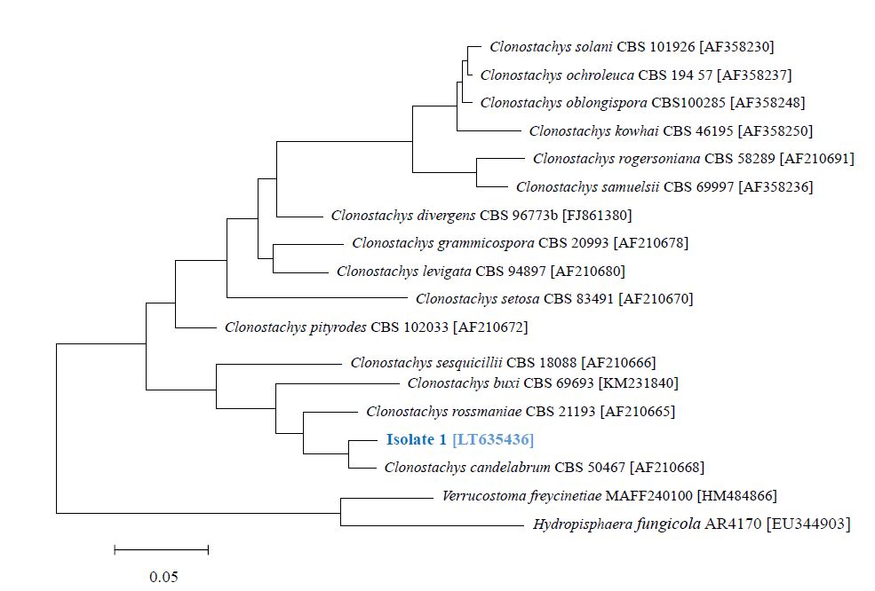
Bruns TD, Fogel R, White TJ, et al. (1990) Amplification and sequencing of DNA from fungal herbarium specimens. Mycologia 82: 175–184. doi: 10.2307/3759846
![]() |
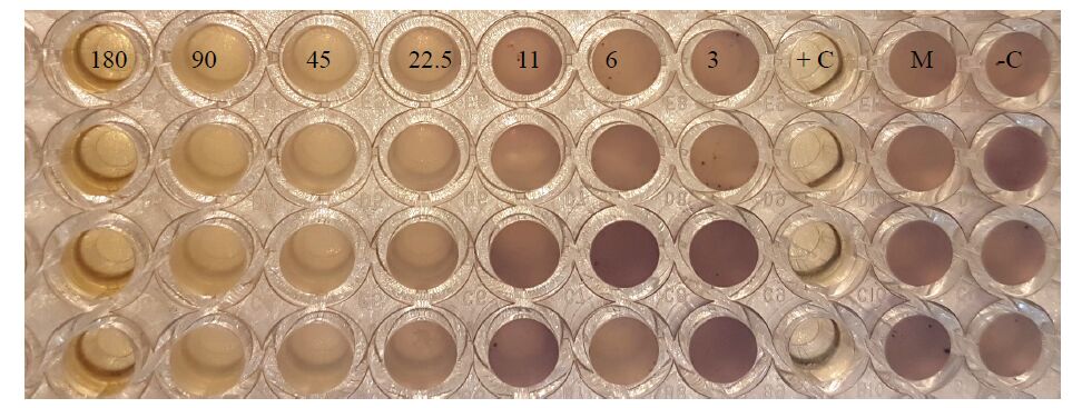
[20] | O'Toole GA (2011) Microtiter dish biofilm formation assay. J Vis Exp 47: e2437–e2437. |
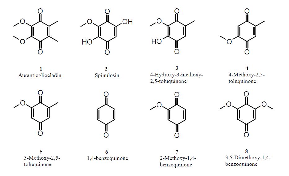
[21] | Franke C, Krohn K (2008) Aurantiogliocladin, In: Roth L, Rupp G, Roth collection of natural products data: concise descriptions and spectra , Weinheim, John Wiley & Sons. |
[22] |
Brian PW, Curtis PJ, Howland SR, et al. (1951) Three new antibiotics from a species of Gliocladium. Experientia 7: 266–267. doi: 10.1007/BF02154546
![]() |
[23] | Vischer EB (1953) The structures of aurantio-and rubro-gliocladin and gliorosein. J Chem Soc (Resumed) , 815–820. |
[24] | Bentley R, Lavate WV (1965) Studies on Coenzyme Q. The biosynthesis of aurantiogliocladin and coenzyme Q in molds. J Biol Chem 240: 532–540. |
[25] |
Pettersson G (1965) New phenolic metabolites from Gliocladium roseum. Acta Chem Scand 19:414–420. doi: 10.3891/acta.chem.scand.19-0414
![]() |
[26] |
Ayers S, Zink DL, Mohn K, et al. (2010). Anthelmintic constituents of Clonostachys candelabrum. J Antibiotics 63:119–122. doi: 10.1038/ja.2009.131
![]() |
[27] |
Mozaina K, Cantrell CL, Mims AB, et al. (2008) Activity of 1,4-benzoquinones against Formosan subterranean termites (Coptotermes formosanus ).J Agric Food Chem 56:4021–4026. doi: 10.1021/jf800331r
![]() |
[28] | Likhovidov VE, Isangalin FS, Naumov AN, et al. (2010) Agents against mosquitos. Russ patent , RU 2391389 C2 20100610. |
[29] | Klink JW, Dropkin VH, Mitchell JE (1970) Studies on the host-finding mechanisms of Neotylenchus linfordi. J Nematol 2:106–117. |
[30] |
Birkinshaw JH, Raistrick H (1931) On a new methoxy-dihydroxy-toluquinone produced from glucose by species of Penicillium of the P. spinulosum series.Phil Trans Roy Soc London. B 220: 245–254. doi: 10.1098/rstb.1931.0023
![]() |
[31] |
Petterson G (1963) Toluquinones from Aspergillus fumigatus. Acta Chem Scand 17:1771–1776. doi: 10.3891/acta.chem.scand.17-1771
![]() |
[32] | Lauer U, Anke T, Hansske F (1991) Antibiotics from basidiomycetes. XXXVIII. 2-Methoxy-5- methyl-1,4-benzoquinone, a thromboxane A2 receptor antagonist from Lentinus adhaerens. J Antibiot 44:59–65. |
[33] |
Attygalle AB, Xu SC, Meinwald J, et al. (1993). Defensive secretion of the millipede Floridobolus penneri. J Nat Prod 56:1700–1706. doi: 10.1021/np50100a007
![]() |
[34] | Nishina A, Uchibori T (1991) Antimicrobial activity of 2, 6-dimethoxy-p-benzoquinone, isolated from thick-stemmed bamboo, its analogs. Agric Biol Chem 55:2395–2398. |
[35] |
Anchel M, Hervey A, Kavanagh F, et al. (1948) Antibiotic substances from Basidiomycetes III. Coprinus similis and Lentinus degener. Proc Nat Acad Sci 34:498–502. doi: 10.1073/pnas.34.11.498
![]() |
[36] | Sood RS, Roy K, Reddy GCS, et al. (1982) 3-Methoxy-2, 5-toluquinone from Aspergillus sp. HPL Y-30,212. Fermentation, isolation, characterization and biological properties. J Antibiot 35:985–987. |
[37] | Oxford AE (1942) Bacteriostatic powers of the methyl ethers of fumigatin and spinulosin and other hydroxy-, methoxy- and hydroxymethoxy-derivatives of toluquinone and benzoquinone. Chem Ind 61:189–192. |
[38] |
Lana EJ, Carazza F, Takahashi JA (2006) Antibacterial evaluation of 1, 4-benzoquinone derivatives. J Agric Food Chem 54:2053–2056. doi: 10.1021/jf052407z
![]() |
[39] |
Estrela AB, Abraham W-R (2010) Combining biofilm-controlling compounds and antibiotics as a promising new way to control biofilm infections. Pharmaceuticals 3:1374–1393. doi: 10.3390/ph3051374
![]() |
[40] |
Wargo MJ, Hogan DA (2006) Fungal-bacterial interactions: a mixed bag of mingling microbes. Curr Opin Microbiol 9: 359–364. doi: 10.1016/j.mib.2006.06.001
![]() |
1. | Xianting Wang, Yun-guang Lu, Richard De la cruz, Guoqiao You, Global Solutions to a Hydrodynamic Model for Semiconductors with Velocity Relaxation, 2023, 43, 0252-9602, 975, 10.1007/s10473-023-0226-0 |