Forkhead box Q1 (FOXQ1) is a nuclear transcription factor that controls the transcriptional activity of downstream genes to exert biological effects. Since its regulatory role in colorectal cancer (CRC) is unknown, we correlated RNA-seq and ATAC-seq sequencing data from the Cancer Genome Atlas Program (TCGA), the Gene Expression Omnibus (GEO), and other databases with FOXQ1 knockdown data from our group and normal DLD1-CRC cell lines. First, we analyzed FOXQ1 gene expression across multiple databases and datasets and found significant differences in FOXQ1 gene expression in most tumors. In addition, we performed an extension analysis of the FOXQ1 gene at different levels and found a close relationship between the FOXQ1 gene and immunity. Then, based on the FOXQ1 gene, we collected its target genes and obtained a total of 107 genes that met the regulatory trend. After a series of target gene analyses, we obtained three key genes (SERPINA1, MYL9, and CFTR). Moreover, an enrichment analysis, an independent prognostic analysis, and an immune-related analysis were performed around FOXQ1 and its target genes. After knocking down FOXQ1 protein in SW480 cells, the SERPINA1 and MYL9 proteins were significantly altered, though the CFTR protein was not significantly changed. These results provide bioinformatics data that support studying and exploring the FOXQ1 gene and its target genes in CRC.
Citation: Yuxiang Zou, Jialong Qi, Hui Tang. Regulatory role of FOXQ1 gene and its target genes in colorectal cancer[J]. AIMS Medical Science, 2024, 11(3): 232-247. doi: 10.3934/medsci.2024018
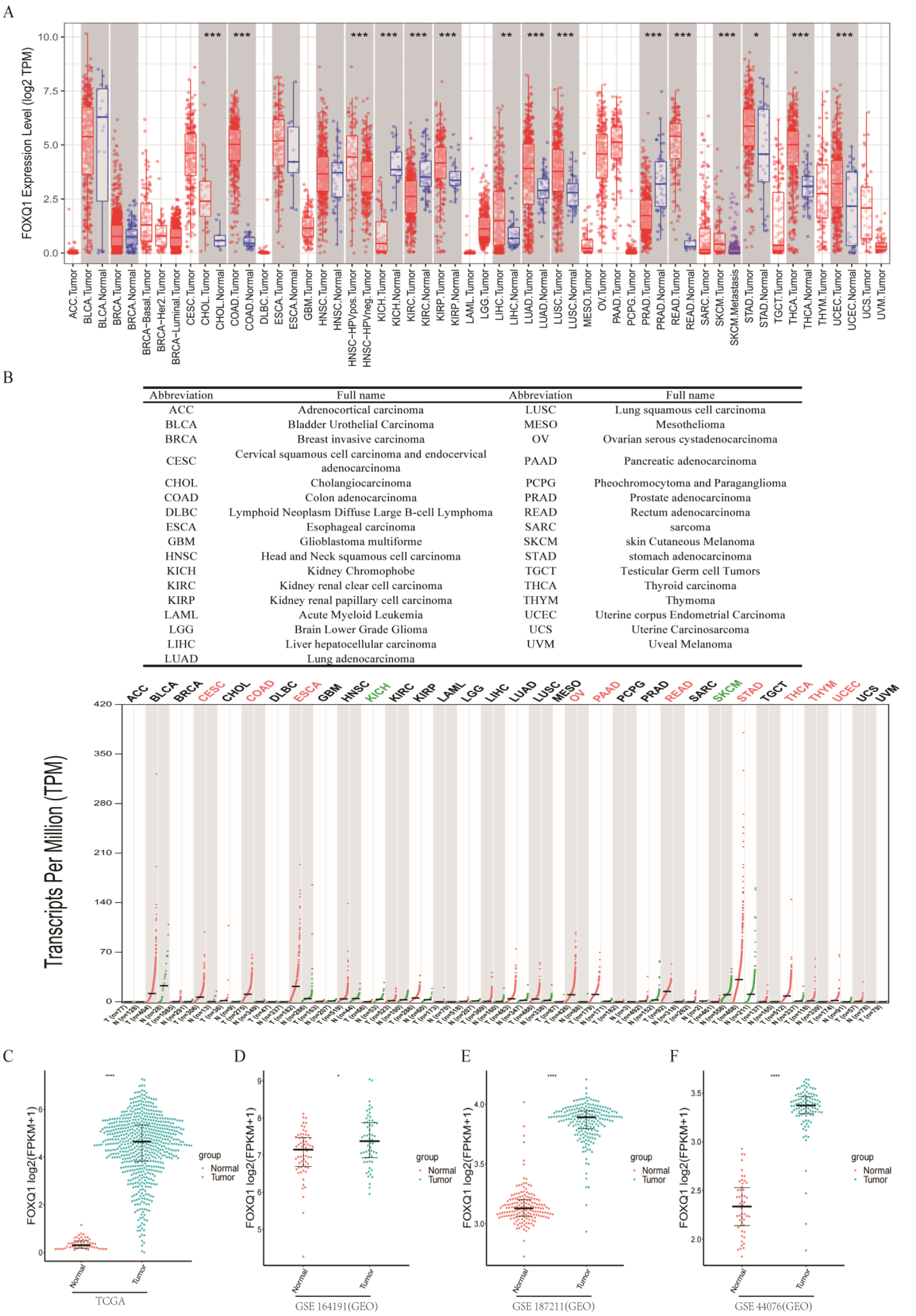
Forkhead box Q1 (FOXQ1) is a nuclear transcription factor that controls the transcriptional activity of downstream genes to exert biological effects. Since its regulatory role in colorectal cancer (CRC) is unknown, we correlated RNA-seq and ATAC-seq sequencing data from the Cancer Genome Atlas Program (TCGA), the Gene Expression Omnibus (GEO), and other databases with FOXQ1 knockdown data from our group and normal DLD1-CRC cell lines. First, we analyzed FOXQ1 gene expression across multiple databases and datasets and found significant differences in FOXQ1 gene expression in most tumors. In addition, we performed an extension analysis of the FOXQ1 gene at different levels and found a close relationship between the FOXQ1 gene and immunity. Then, based on the FOXQ1 gene, we collected its target genes and obtained a total of 107 genes that met the regulatory trend. After a series of target gene analyses, we obtained three key genes (SERPINA1, MYL9, and CFTR). Moreover, an enrichment analysis, an independent prognostic analysis, and an immune-related analysis were performed around FOXQ1 and its target genes. After knocking down FOXQ1 protein in SW480 cells, the SERPINA1 and MYL9 proteins were significantly altered, though the CFTR protein was not significantly changed. These results provide bioinformatics data that support studying and exploring the FOXQ1 gene and its target genes in CRC.

| [1] |
Mármol I, Sánchez-de-Diego C, Pradilla Dieste A, et al. (2017) Colorectal carcinoma: A general overview and future perspectives in colorectal cancer. Int J Mol Sci 18: 197. https://doi.org/10.3390/ijms18010197 
|
| [2] |
Bieller A, Pasche B, Frank S, et al. (2001) Isolation and characterization of the human forkhead gene FOXQ1. DNA Cell Biol 20: 555-561. https://doi.org/10.1089/104454901317094963
|
| [3] |
Kaneda H, Arao T, Tanaka K, et al. (2010) FOXQ1 is overexpressed in colorectal cancer and enhances tumorigenicity and tumor growth. Cancer Res 70: 2053-2063. https://doi.org/10.1158/0008-5472.CAN-09-2161
|
| [4] | Lin L, Miller CT, Contreras JI, et al. (2002) The hepatocyte nuclear factor 3 alpha gene, HNF3alpha (FOXA1), on chromosome band 14q13 is amplified and overexpressed in esophageal and lung adenocarcinomas. Cancer Res 62: 5273-5279. |
| [5] |
Li J, Vogt PK (1993) The retroviral oncogene qin belongs to the transcription factor family that includes the homeotic gene fork head. P Natl Acad Sci Usa 90: 4490-4494. https://doi.org/10.1073/pnas.90.10.4490
|
| [6] |
Koo CY, Muir KW, Lam EW (2012) FOXM1: From cancer initiation to progression and treatment. Biochim Biophys Acta-Gene Regul Mech 1819: 28-37. https://doi.org/10.1016/j.bbagrm.2011.09.004
|
| [7] |
Christensen J, Bentz S, Sengstag T, et al. (2013) FOXQ1, a novel target of the Wnt pathway and a new marker for activation of Wnt signaling in solid tumors. PloS One 8: e60051. https://doi.org/10.1371/journal.pone.0060051
|
| [8] |
Ellis LM, Hicklin DJ (2008) VEGF-targeted therapy: mechanisms of anti-tumour activity. Nat Rev Cancer 8: 579-591. https://doi.org/10.1038/nrc2403
|
| [9] |
Ross JB, Huh D, Noble LB, et al. (2015) Identification of molecular determinants of primary and metastatic tumour re-initiation in breast cancer. Nat Cell Biol 17: 651-664. https://doi.org/10.1038/ncb3148
|
| [10] |
Feng J, Zhang X, Zhu H, et al. (2012) FoxQ1 overexpression influences poor prognosis in non-small cell lung cancer, associates with the phenomenon of EMT. PloS One 7: e39937. https://doi.org/10.1371/journal.pone.0039937
|
| [11] |
Meng F, Speyer CL, Zhang B, et al. (2015) PDGFRα and β play critical roles in mediating Foxq1-driven breast cancer stemness and chemoresistance. Cancer Res 75: 584-593. https://doi.org/10.1158/0008-5472.CAN-13-3029
|
| [12] |
Wattenberg LW (1977) Inhibition of carcinogenic effects of polycyclic hydrocarbons by benzyl isothiocyanate and related compounds. J Natl Cancer Inst 58: 395-398. https://doi.org/10.1093/jnci/58.2.395
|
| [13] |
Sehrawat A, Kim SH, Vogt A, et al. (2013) Suppression of FOXQ1 in benzyl isothiocyanate-mediated inhibition of epithelial-mesenchymal transition in human breast cancer cells. Carcinogenesis 34: 864-873. https://doi.org/10.1093/carcin/bgs397
|
| [14] |
Pott S, Lieb JD (2015) Single-cell ATAC-seq: strength in numbers. Genome Biol 16: 172. https://doi.org/10.1186/s13059-015-0737-7
|
| [15] | Buenrostro JD, Wu B, Chang HY, et al. (2015) ATAC-seq: A method for assaying chromatin accessibility genome-wide. Curr Protoc Mol Biol 10. https://doi.org/10.1002/0471142727.mb2129s109 |
| [16] |
Collins CB, Aherne CM, Ehrentraut SF, et al. (2013) Alpha-1-antitrypsin therapy ameliorates acute colitis and chronic murine ileitis. Inflamm Bowel Dis 19: 1964-1973. https://doi.org/10.1097/MIB.0b013e31829292aa
|
| [17] |
Fournier N, Fabre A (2022) Smooth muscle motility disorder phenotypes: A systematic review of cases associated with seven pathogenic genes (ACTG2, MYH11, FLNA, MYLK, RAD21, MYL9 and LMOD1). Intractable Rare Dis Res 11: 113-119. https://doi.org/10.5582/irdr.2022.01060
|
| [18] |
Thiagarajah JR, Verkman AS (2003) CFTR pharmacology and its role in intestinal fluid secretion. Curr Opin Pharmacol 3: 594-599. https://doi.org/10.1016/j.coph.2003.06.012
|


Figures(6)

Yuxiang Zou, Jialong Qi, Hui Tang. Regulatory role of FOXQ1 gene and its target genes in colorectal cancer[J]. AIMS Medical Science, 2024, 11(3): 232-247. doi: 10.3934/medsci.2024018


 DownLoad: